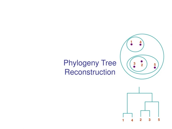
Phylogeny Tree Reconstruction
1. 4. 3. 5. 2. 5. 2. 3. 1. 4. Phylogeny Tree Reconstruction. Final Exam. 24-hour, takehome exam More straight-forward questions than in homeworks Please email Michael and Serafim by Friday, with your preference of day to take exam


Phylogeny Tree Reconstruction
E N D
Presentation Transcript
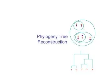
1 4 3 5 2 5 2 3 1 4 Phylogeny Tree Reconstruction
Final Exam • 24-hour, takehome exam • More straight-forward questions than in homeworks • Please email Michael and Serafim by Friday, with your preference of day to take exam • Exam starts Sunday, …, Thursday noon; ends Monday, ..., Friday noon
Number of labeled unrooted tree topologies • How many possibilities are there for leaf 4? 2 1 4 4 4 3
Number of labeled unrooted tree topologies • How many possibilities are there for leaf 4? For the 4th leaf, there are 3 possibilities 2 1 4 3
Number of labeled unrooted tree topologies • How many possibilities are there for leaf 5? For the 5th leaf, there are 5 possibilities 2 1 4 5 3
Number of labeled unrooted tree topologies • How many possibilities are there for leaf 6? For the 6th leaf, there are 7 possibilities 2 1 4 5 3
Number of labeled unrooted tree topologies • How many possibilities are there for leaf n? For the nth leaf, there are 2n – 5 possibilities 2 1 4 5 3
Number of labeled unrooted tree topologies • #unrooted trees for n taxa: (2n-5)*(2n-7)*...*3*1 = (2n-5)! / [2n-3*(n-3)!] • #rooted trees for n taxa: (2n-3)*(2n-5)*(2n-7)*...*3 = (2n-3)! / [2n-2*(n-2)!] 2 1 N = 10 #unrooted: 2,027,025 #rooted: 34,459,425 N = 30 #unrooted: 8.7x1036 #rooted: 4.95x1038 4 5 3
Search through tree topologies: Branch and Bound Observation: adding an edge to an existing tree can only increase the parsimony cost Enumerate all unrooted trees with at most n leaves: [i3][i5][i7]……[i2N–5]] where each ik can take values from 0 (no edge) to k At each point keep C = smallest cost so far for a complete tree Start B&B with tree [1][0][0]……[0] Whenever cost of current tree T is > C, then: • T is not optimal • Any tree extending T with more edges is not optimal: Increment by 1 the rightmost nonzero counter
Bootstrapping to get the best trees Main outline of algorithm • Select random columns from a multiple alignment – one column can then appear several times • Build a phylogenetic tree based on the random sample from (1) • Repeat (1), (2) many (say, 1000) times • Output the tree that is constructed most frequently
Probabilistic Methods A more refined measure of evolution along a tree than parsimony P(x1, x2, xroot | t1, t2) = P(xroot) P(x1 | t1, xroot) P(x2 | t2, xroot) If we use Jukes-Cantor, for example, and x1 = xroot = A, x2 = C, t1 = t2 = 1, = pA¼(1 + 3e-4α) ¼(1 – e-4α) = (¼)3(1 + 3e-4α)(1 – e-4α) xroot t1 t2 x1 x2
Probabilistic Methods xroot = x2N-1 • If we know all internal labels xu, P(x1, x2, …, xN, xN+1, …, x2N-1 | T, t) = P(xroot)jrootP(xj | xparent(j), tj, parent(j)) • Usually we don’t know the internal labels, therefore P(x1, x2, …, xN | T, t) = xN+1 xN+2 … x2N-1P(x1, x2, …, x2N-1 | T, t) xu x2 xN x1
Computing the Likelihood of a Tree xk • Define P(Lk | a): probability of subtree rooted at xk, given that xk = a • Then, P(Lk | a) = (bP(Li | b) P(b | a, tki))(cP(Lj | c) P(c | a, tki)) tkj tki xj xi
Felsenstein’s Likelihood Algorithm To calculate P(x1, x2, …, xN | T, t) Initialization: Set k = 2N – 1 Recursion: Compute P(Lk | a) for all a If k is a leaf node: Set P(Lk | a) = 1(a = xk) If k is not a leaf node: 1. Compute P(Li | b), P(Lj | b) for all b, for daughter nodes i, j 2. Set P(Lk | a) = b,cP(b | a, tki)P(Li | b) P(c | a, tkj) P(Lj | c) Termination: Likelihood at this column = P(x1, x2, …, xN | T, t) = aP(L2N-1 | a)P(a)
Probabilistic Methods Given M (ungapped) alignment columns of N sequences, • Define likelihood of a tree: L(T, t) = P(Data | T, t) = m=1…M P(x1m, …, xnm, T, t) Maximum Likelihood Reconstruction: • Given data X = (xij), find a topology T and length vector t that maximize likelihood L(T, t)
Nanopore Sequencing http://www.mcb.harvard.edu/branton/index.htm
Nanopore Sequencing http://www.mcb.harvard.edu/branton/index.htm
Nanopore Sequencing—Assembly • Resulting reads are likely to look different than Sanger reads: • Long (perhaps 10,000bp-1,000,000bp) • High error rate (perhaps 10% – 30%) • Two colors? • A/ CTG • AT/ CG • AG/ CT • How can we assemble under such conditions?
Pyrosequencing on a chip • Mostafa Ronaghi, Stanford Genome Technologies Center • 454 Life Sciences
Pyrosequencing—Assembly • Resulting reads are likely to look different than Sanger reads: • Short (currently 100 to 200 bp) • Low error rates, except in homopolymeric runs (AAA…, CCC…, etc) • Currently, not known how to do paired reads on a chip ?