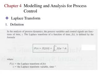
4 . Laplace Transform Methods

1. 4. Laplace Transform Methods 4.1 Linear systems 4.1.1 Linear differential equations 4.1.2 A fundamental property 4.2 The Laplace transform 4.2.1Definition 4.2.2 Laplace transforms of common functions 4.2.3 Properties of the Laplace transform 4.3 Modelling in the Laplace domain 4.3.1The transfer function 4.3.2Working with transfer functions 4.4 Applying the inverse Laplace transform 4.4.1Solving linear differential equations 4.4.2 Partial fraction expansion 4.5 Table of Laplace transforms Process Dynamics and Control

2. 4.1 Linear systems • In practice, all real processes (systems) are to some degree nonlinear. However, there are several reasons why we want to study linear systems. • It is often difficult to include the right nonlinearity in a model; a linear model might be the best available approximation. • A system operating close to a stationary operating point — as controlled systems tend to do — often behaves as a linear system. • There are powerful methods based on linear algebra and operator theory for analysis, synthesis and design of linear systems. • As we have seen, differential equations • give a mathematical description of continuous-time dynamical systems • describe how a given variable, the output, depends on one or several other variables, inputs • Linear DEs are therefore suitable for describing linear continuous-time systems mathematically. Process Dynamics and Control

3. 4.1 Linear systems 4.1.1 Linear differential equations • A linear ODE has the general form • (4.1) • is the outputfrom the system, is the input to the system. • , the order of the highest output derivative, is the system order. • The system is proper if , it is strictly proper if ; physical systems are practically always proper (but an ideal controller might be nonproper). • The coefficients are system parameters that completely characterize the properties of the system. • The system parameters can be rescaled (if desired) by multiplying (or dividing) them all by the same factor. Rescaling to get • is always possible (if , the system is not :th order) • is possible if the static gain is nonzero (which usually applies) Process Dynamics and Control

4. 4.1.1 Linear differential equations • If the system is proper, we can always use as the order of the highest derivative of the input by letting the coefficients be zero in • Thus, we can without loss of generality write • (4.2) • Note how the subscripts of the coefficients are related to the order of the corresponding time derivative. (This will be useful later.) Process Dynamics and Control

5. 4.1 Linear systems 4.1.2 A fundamental property For linear systems, the principle of superposition applies. Assume that (4.3a) (4.3b) are two solutions to (4.2). According to the principle of superposition, the input (4.4) where and are arbitrary constants, gives the solution (4.5) For a linear system with more than one input, this implies that we can consider one input at a time. The combined effect of several inputs is then obtained by combining the respective outputs in the same way. This is a reason why it is (usually) sufficient to include only one input in the DE (4.1) or (4.2). Process Dynamics and Control

6. 4.2 The Laplace transform • It is possible to solve the linear ODE (4.1) or (4.2) “analytically” using basic mathematics if • the system parameters are constant • the inputhas a reasonable simple form • The full solution, i.e. the function , is obtained as the sum of • a particular solution (any solution satisfying the DE) • the general solution to the corresponding autonomous DE () • However, this way of solving DEs is cumbersome: • the mathematics tend to be complicated for systems of high order • there are no convenient short-cuts do deal with systems composed of simple subsystems • The Laplace transform offers a practical way of solving linear DEs. Furthermore, it plays a fundamental role in analysis, synthesis, and design of linear systems. It is especially useful for systems with one output (and one input). Process Dynamics and Control

7. 4.2 The Laplace transform 4.2.1 Definition • The signals in dynamical systems are functions of time. Consider a fairly arbitrary function . For “technical reasons” concerning the Laplace transform we need to assume that • for , can be integrated for . • The Laplace transform of such a time function is defined by the integral • (4.6) • where is a complex variable, whose real part has to be large enough for the integral to have a finite value. • is a function in the time domain. • is a function in the Laplace domain or domain. • It is recommended to use small (lower-case) letters for functions in the time domain and the corresponding large (upper-case) letter for a function in the Laplace domain. • This recommendation is not always obeyed; we could use the same letter followed by the domain variable or as argument (e.g. and ). Process Dynamics and Control

8. 4.2.1 Definition • The inverse Laplace transform • In order for the Laplace transform to be useful, it is necessary to also be able to transform the other way, i.e. to calculate the time function that corresponds to a given Laplace function . • Formally, this can be done by means of the integral formula • , (4.7) • where is the imaginary unit and is a real number large enough so that is finite for all . • In practical calculations • we do not need (4.7) • we seldom need (4.6) • because we will use tabulated Laplace transform/time domain function pairs. However, we will need to apply • the superposition principle • partial fraction expansion (section 4.4.2) • to be able to use tabulated function relationships. Process Dynamics and Control

9. 4.2 The Laplace transform 4.2.2 Laplace transforms of common functions • A rectangular pulse • Fig. 4.1. A rectangular pulse. • (4.8) • A unit pulse has the area 1, i.e. . The Laplace transform of the unit pulse is thus • (4.9) • A rectangular pulse has a • constant amplitude (height) • given pulse length • It is assumed to start at . • By means of the Laplace transform • definition (4.6) we can derive Process Dynamics and Control

10. 4.2.2 Laplace transforms of common functions • The unit impulse — Dirac’s delta function • An impulse is defined as a (rectangular) pulse, whose • pulse length • amplitude • is finite • For the unit impulse, denoted , • (with some unit according to the application) • The Laplace transform of the unit impulse can be obtained by letting in the Laplace transform of the unit pulse. A Taylor series expansion then gives • (4.10) • Impulses are important in many practical applications. Input signals of very short duration can usually be approximated by impulses. E.g. • voltage and current pulses in electrical systems • sudden forces in mechanical systems, e.g. wind gusts • injection of tracers in medical and process technical applications Process Dynamics and Control

11. 4.2.2 Laplace transforms of common functions • A unit step • A step function can be considered a rectangular pulsewith • infinite pulse length • For aunit step, denoted , • (with some unit) • The Laplace transform of a unit step can be derived • by letting in the Laplace transform of a pulse • with . A Taylor series expansion gives • (4.11) • A unit ramp • A ramp function is a function whose value changes • linearly with time. For a unit ramp, denoted , the • slope coefficient is , i.e. , . • The Laplace transform of the unit ramp can be derived • from the definition (4.6). Integration by parts gives • (4.12) Process Dynamics and Control

12. 4.2.2 Laplace transforms of common functions • Relationships between the simple unit functions • Consider the unit impulse, unit step, and unit ramp in Fig. 4.2. • the impulse is the time derivative of the step function • the step function is the time derivate of the ramp function • Mathematically: • , • In the Laplace domainwe have derived the relationships: • , • This means that • a time derivative corresponds to multiplication by in the -domain • thus, a time integral corresponds to division by in the -domain • Fig. 4.2. A unit impulse, unit step, and unit ramp. Process Dynamics and Control

13. 4.2.2 Laplace transforms of common functions • Exponential function • An exponential function is defined , . If • , the function is exponentially decaying • , the function is exponentially increasing • The Laplace transform can be derived from the • definition (4.6) • (4.13) • It is not clear from the final result, but the integral • exists (is finite) if and only if This is a limiting restriction mainly if , i.e. if the function is exponentially increasing. Such a function is unstable, because it approaches infinity as time goes towards infinity. Process Dynamics and Control

14. 4.2.2 Laplace transforms of common functions • Sine and cosine functions • The sine function (with amplitude one) is de- • fined , , where is the • oscillation frequency in radians per time unit. • The Laplace transform can be derived using • integration by parts, defined • By applying partial integration twice to the definition (4.6), we can derive • (4.14) • The cosine function (amplitude one) is defined, . Similarly as above, we can derive • (4.15) • We could have derived (4.15) more easily by • observing that • and using . Process Dynamics and Control

15. 4.2 The Laplace transform 4.2.3 Properties of the Laplace transform • Superposition • If and • then (4.16) • (4.17) • where and are arbitrary constants. • This means that we can easily calculate the • Laplace transform of the linear combination according to (4.16) • inverse Laplace transform of according to (4.17) • if we know the Laplace transforms of (the simpler functions) and . Process Dynamics and Control

16. 4.2.3 Properties of the Laplace transform • Derivatives • If , then the Laplace transform of the first-order time derivative is given by • (4.18) • where • i.e. is the initial value of the time domain function when approaches from the left. Left or right make a difference if has adiscontinuity at (e.g. a step function). • The Laplace transform of an :th order derivative is • (4.19) • where , , … are the values of , , … when . • Note that all initial values are for systems, where the variables are deviations from a steady-state operating point. Process Dynamics and Control

17. 4.2.3 Properties of the Laplace transform • Integrals • If , the Laplace transform of the time integral of is given by • (4.20) • For a multiple integral, the Laplace transform is • (4.21) • Note that initial values are not an issue in this case. Process Dynamics and Control

18. 4.2.3 Properties of the Laplace transform • Integrals • If , the Laplace transform of the time integral of is given by • (4.20) • For a multiple integral, the Laplace transform is • (4.21) • Note that initial values are not an issue in this case. • Damping • If , the Laplace transform of an exponentially damped function is given by • (4.22) • Note that it is required that , which is a limiting restriction if . In practice, (otherwise there is no damping). Process Dynamics and Control

19. 4.2.3 Properties of the Laplace transform • Time delay • If , the Laplace transform of the function , i.e. the function delayed by time units, is given by • (4.23) • Fig. 4.3. Undelayed and delayed time function. Process Dynamics and Control

20. 4.2.3 Properties of the Laplace transform • Exercise 4.1 • Determine the Laplace transform of the function • Validate the result by means of the initial and final value theorems. • Exercise 4.2 • Determine the time function whose Laplace transform is • Validate the result by means of the initial and final value theorems. • Exercise 4.3 • Determine the Laplace transform of the • delayed saw tooth pulse in the figure. Process Dynamics and Control

21. 4.2.3 Properties of the Laplace transform • Limit theorems • In general • small values of the time variable corresponds to large values of the Laplace variable • and vice versa • However, there is no exact relationship between time the Laplace variable, except for two limit conditions. They are useful for calculating the initial and final steady-state values of a time function whose Laplace transform is known without doing an inverse Laplace transformation. • The initial value theorem • If , where is strictly proper, • (4.24) • Here means that approaches zero from the positive side of . • The final value theorem • If , where is bounded for all , • (4.25) Process Dynamics and Control

22. 4.5 Table of Laplace transforms • From Tore Gustafsson: Ingenjörsmatematisk formelsamling, 1999–2009. Process Dynamics and Control

23. 4.5 Table of Laplace transforms Process Dynamics and Control

24. 4.5 Table of Laplace transforms Process Dynamics and Control

25. 4.5 Table of Laplace transforms Process Dynamics and Control

26. 4.5 Table of Laplace transforms Process Dynamics and Control

27. 4.5 Table of Laplace transforms Process Dynamics and Control

28. 4.5 Table of Laplace transforms Process Dynamics and Control

29. 4.5 Table of Laplace transforms Process Dynamics and Control