Logarithms
Logarithms. Properties and Uses. Some background. Review section 1.6 of Feinstein and Thomas, pp. 14-19. A logarithm (generally called the “log” of a number) is the “power to which a given base must be raised to equal that number” (Feinstein and Thomas, p. 16).

Logarithms
E N D
Presentation Transcript
Logarithms Properties and Uses
Some background • Review section 1.6 of Feinstein and Thomas, pp. 14-19. • A logarithm (generally called the “log” of a number) is the “power to which a given base must be raised to equal that number” (Feinstein and Thomas, p. 16). • Common bases: Base 10 and Base e.
Examples • Base 10 logarithms: • 10 * 10 = 100. So 10 squared equals 100 or 102 = 100. So the log of 100 to the base 10 equals 2. • 10 * 10 * 10 = 1000. So 10 cubed equals 1000 or 103= 1000. So the log of 1000 to the base 10 equals 3. Etc…..
Base 10 Logarithm Examples CASE NUMBER BASE 10 LOG 1.000 1.000 0.000 2.000 10.000 1.000 3.000 100.000 2.000 4.000 200.000 2.301 5.000 500.000 2.699 6.000 1000.000 3.000 7.000 5000.000 3.699 8.000 10000.000 4.000 9.000 15000.000 4.176 10.000 30000.000 4.477
Properties of Logarithms • A proportionate change in the original number becomes an arithmetic change in the logarithm. • The base 10 logarithm of 10 is 1. The base 10 log of 100 is 2. The base 100 log of 1000 is 3. • The tenfold increase from 1 to 10, 10 to 100 and 100 to 1000, is a 1 unit increase in the base 10 log, from 1 to 2 to 3.
Properties of Logarithms • The properties of logarithms make them useful for the analysis of growth (or decay). • Economists remeasure series which exhibit strong growth patterns in logarithms to capture the proportionate change as an arithmetic change. • OLS regression can then be used to explore relationships.
Base 10 Logarithm Examples VAR00008 LOGVAR 1 1.000 1.000 0.000 2 2.000 10.000 1.000 3 3.000 100.000 2.000 4 4.000 200.000 2.301 5 5.000 500.000 2.699 6 6.000 1000.000 3.000 7 7.000 5000.000 3.699 8 8.000 10000.000 4.000 9 9.000 15000.000 4.176 10 10.000 30000.000 4.477
Properties of Logarithms • The most common base used is base e, or natural logarithm, which is also is written ln. • “e” is a numeric constant (like pi) which formally is equal to the limit of the sequence of terms (1 + 1/N)N as the integer N grows larger and larger. • An approximation when N = 10,000 is 2.718145. [that is (10,001/10,000)10,000]
Log and Anti Log Transformations • Scientific calculators and statistical programs have functions to transform a number into its log value. • Log values can be converted back to the original value by using the anti log or the exponentiating function.
Antilog or exponentiating function Natural log function
Simple and Compound Interest • Simple interest formula: y = a + b*x where • Y = final value • a = initial value • b = interest rate • x = time • So, after 10 years, a $100 investment with simple interest at the rate of 2%: • Y = 100 + 2 * 10 = $120
Example: Compound Interest Future value = Present Value * (1 + i)n • Future value = Product of Present value times (1 plus the interest rate raised to the number of time periods). • So if present value = $100, and the interest rate is 2% (.02) and the time period is one year, the future value after a year is $102. • After two years, the future value is $102 * 1.02 or $104.04.
Compound Interest example • Year 1: F = (P + r*P) • Year 2: F = (P + r*P) + r (P + r*P) • Year 3: F = ((P * r*P) + r (P + r*P)) + • r* ((P + r*P) + r (P + r*P)) • or • Year 1: F = 100 + .02*100 = 102 • Year 2: F = 102 + .02 (102) = 104.04 • Year 3: F = 104.04 + .02 (104.04) = 106.12
Compound Interest example • Year 1: F = (P + r*P) • Year 2: F = (P + r*P) + r (P + r*P) • Year 3: F = ((P * r*P) + r (P + r*P)) + • r* ((P + r*P) + r (P + r*P)) • or • Year 1: F = P (1 +r) • Year 2: F = P (1 + 2 r + r2) = P (r+1)2 • Year 3: F = P (r+1)3
Example of Interest Calculations: $100 invested at 2% and 6% over 10 time periods SIMPLE COMPND TIME LN COMPND LOG COMPND SIMPLE6 COMPND6 1 102.000 102.000 1.000 4.625 2.009 106.000 106.000 2 104.000 104.040 2.000 4.645 2.017 112.000 112.360 3 106.000 106.120 3.000 4.665 2.026 118.000 119.100 4 108.000 108.240 4.000 4.684 2.034 124.000 126.250 5 110.000 110.410 5.000 4.704 2.043 130.000 133.820 6 112.000 112.620 6.000 4.724 2.052 136.000 141.850 7 114.000 114.870 7.000 4.744 2.060 142.000 150.360 8 116.000 117.170 8.000 4.764 2.069 148.000 159.380 9 118.000 119.510 9.000 4.783 2.077 154.000 168.950 10 120.000 121.900 10.000 4.803 2.086 160.000 179.080