Download
1 / 34
340 likes | 357 Vues
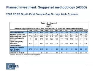
Lecture 8. 11. Aggregate Demand in the Goods and Money Markets. LECTURE OUTLINE. Planned Investment and the Interest Rate Other Determinants of Planned Investment Planned Aggregate Expenditure and the Interest Rate Equilibrium in Both the Goods and Money Markets

E N D
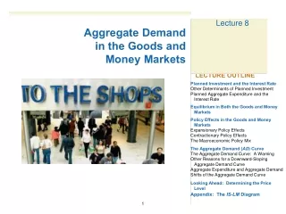
Lecture 8 11 Aggregate Demandin the Goods andMoney Markets LECTURE OUTLINE Planned Investment and the Interest Rate Other Determinants of Planned Investment Planned Aggregate Expenditure and theInterest Rate Equilibrium in Both the Goods and MoneyMarkets Policy Effects in the Goods and MoneyMarketsExpansionary Policy Effects Contractionary Policy Effects The Macroeconomic Policy Mix The Aggregate Demand (AD) CurveThe Aggregate Demand Curve: A WarningOther Reasons for a Downward-Sloping Aggregate Demand CurveAggregate Expenditure and Aggregate DemandShifts of the Aggregate Demand Curve Looking Ahead: Determining the Price Level Appendix: The IS-LM Diagram
Aggregate Demand in the Goods and Money Markets goods market The market in which goods and services are exchanged and in which the equilibrium level of aggregate output is determined. money market The market in which financial instruments are exchanged and in which the equilibrium level of the interest rate is determined.
Planned Investment and the Interest Rate FIGURE 12.1 Planned Investment Schedule Planned investment spending is a negative function of the interest rate. An increase in the interest rate from 3 percent to 6 percent reduces planned investment from I0 to I1.
Planned Investment and the Interest Rate Other Determinants of Planned Investment The assumption that planned investment depends only on the interest rate is obviously a simplification, just as is the assumption that consumption depends only on income. In practice, the decision of a firm on how much to invest depends on, among other things, its expectation of future sales. The optimism or pessimism of entrepreneurs about the future course of the economy can have an important effect on current planned investment. Keynes used the phrase animal spirits to describe the feelings of entrepreneurs, and he argued that these feelings affect investment decisions.
Planned Investment and the Interest Rate Other Determinants of Planned Investment Interest Rates and Investment Spending A recent study by Simon Gilchrist, Fabio Natalucci, and Egon Zakrajsek finds that interest rates have a powerful effect on the behavior of firms.
Planned Investment and the Interest Rate Planned Aggregate Expenditure and the Interest Rate We can use the fact that planned investment depends on the interest rate to consider how planned aggregate expenditure (AE) depends on the interest rate. Recall that planned aggregate expenditure is the sum of consumption, planned investment, and government purchases. AE ≡ C + I + G
Planned Investment and the Interest Rate Planned Aggregate Expenditure and the Interest Rate FIGURE 12.2 The Effect of an Interest Rate Increase on Planned Aggregate Expenditure An increase in the interest rate from 3 percent to 6 percent lowers planned aggregate expenditure and thus reduces equilibrium income from Y0 to Y1.
Planned Investment and the Interest Rate Planned Aggregate Expenditure and the Interest Rate • The effects of a change in the interest rate include: • A high interest rate (r) discourages planned investment (I). • Planned investment is a part of planned aggregate expenditure (AE). • Thus, when the interest rate rises, planned aggregate expenditure (AE) at every level of income falls. • Finally, a decrease in planned aggregate expenditure lowers equilibrium output (income) (Y) by a multiple of the initial decrease in planned investment.
Planned Investment and the Interest Rate Planned Aggregate Expenditure and the Interest Rate Using a convenient shorthand:
Equilibrium in Both the Goods and Money Markets An increase in the interest rate (r) decreases output (Y) in the goods market because an increase in r lowers planned investment. When income (Y) increase, this shifts the money demand curve to the right, which increases the interest rate (r) with a fixed money supply. We can thus write:
Equilibrium in Both the Goods and Money Markets FIGURE 12.3 Links Between the Goods Market and the Money Market Planned investment depends on the interest rate, and money demand depends on aggregate output.
Policy Effects in the Goods and Money Markets Expansionary Policy Effects expansionary fiscal policy An increase in government spending or a reduction in net taxes aimed at increasing aggregate output (income) (Y). expansionary monetary policy An increase in the money supply aimed at increasing aggregate output (income) (Y).
Policy Effects in the Goods and Money Markets Expansionary Policy Effects Expansionary Fiscal Policy: An Increase in Government Purchases (G) or a Decrease in Net Taxes (T) crowding-out effect The tendency for increases in government spending to cause reductions in private investment spending.
Policy Effects in the Goods and Money Markets Expansionary Policy Effects Expansionary Fiscal Policy: An Increase in Government Purchases (G) or a Decrease in Net Taxes (T) FIGURE 12.4 The Crowding-Out Effect An increase in government spending G from G0 to G1 shifts the planned aggregate expenditure schedule from 1 to 2. The crowding-out effect of the decrease in planned investment (brought about by the increased interest rate) then shifts the planned aggregate expenditure schedule from 2 to 3.
Effects of an expansionary fiscal policy: Policy Effects in the Goods and Money Markets Expansionary Policy Effects Expansionary Fiscal Policy: An Increase in Government Purchases (G) or a Decrease in Net Taxes (T) interest sensitivity or insensitivity of planned investment The responsiveness of planned investment spending to changes in the interest rate. Interest sensitivity means that planned investment spending changes a great deal in response to changes in the interest rate; interest insensitivity means little or no change in planned investment as a result of changes in the interest rate.
Effects of an expansionary monetary policy: Policy Effects in the Goods and Money Markets Expansionary Policy Effects Expansionary Monetary Policy: An Increase in the Money Supply
Effects of a contractionary fiscal policy: Policy Effects in the Goods and Money Markets Contractionary Policy Effects Contractionary Fiscal Policy: A Decrease in Government Spending (G) or an Increase in Net Taxes (T) contractionary fiscal policy A decrease in government spending or an increase in net taxes aimed at decreasing aggregate output (income) (Y).
Effects of a contractionary monetary policy: Policy Effects in the Goods and Money Markets Contractionary Policy Effects Contractionary Monetary Policy: A Decrease in the Money Supply contractionary monetary policy A decrease in the money supply aimed at decreasing aggregate output (income) (Y).
The Aggregate Demand (AD) Curve aggregate demand The total demand for goods and services in the economy. aggregate demand (AD) curve A curve that shows the negative relationship between aggregate output (income) and the price level. Each point on the AD curve is a point at which both the goods market and the money market are in equilibrium.
The Aggregate Demand (AD) Curve FIGURE 12.5 The Impact of an Increase in the Price Level on the Economy—Assuming No Changes in G, T, and Ms This figure shows that when P increases, Y decreases.
The Aggregate Demand (AD) Curve FIGURE 12.6The Aggregate Demand (AD) Curve At all points along the AD curve, both the goods market and the money market are in equilibrium. The policy variables G, T, and Ms are fixed.
The Aggregate Demand (AD) Curve The Aggregate Demand Curve: A Warning It is important that you realize what the aggregate demand curve represents. The aggregate demand curve is more complex than a simple individual or market demand curve. The AD curve is not a market demand curve, and it is not the sum of all market demand curves in the economy. To understand what the aggregate demand curve represents, you must understand the interaction between the goods market and the money markets.
The Aggregate Demand (AD) Curve Other Reasons for a Downward-Sloping Aggregate Demand Curve The Consumption Link The consumption link provides another reason for the AD curve’s downward slope. An increase in the price level increases the demand for money, which leads to an increase in the interest rate, which leads to a decrease in consumption (as well as planned investment), which leads to a decrease in aggregate output (income).
The Aggregate Demand (AD) Curve Other Reasons for a Downward-Sloping Aggregate Demand Curve The Consumption Link The initial decrease in consumption (brought about by the increase in the interest rate) contributes to the overall decrease in output. Planned investment does not bear all the burden of providing the link from a higher interest rate to a lower level of aggregate output. Decreased consumption brought about by a higher interest rate also contributes to this effect.
The Aggregate Demand (AD) Curve Other Reasons for a Downward-Sloping Aggregate Demand Curve The Real Wealth Effect real wealth, or real balance, effect The change in consumption brought about by a change in real wealth that results from a change in the price level.
The Aggregate Demand (AD) Curve Aggregate Expenditure and Aggregate Demand At equilibrium, planned aggregate expenditure (AE≡C + I + G) and aggregate output (Y) are equal: equilibrium condition: C + I + G = Y
The Aggregate Demand (AD) Curve Shifts of the Aggregate Demand Curve FIGURE 12.7The Effect of an Increase in Money Supply on the AD Curve An increase in the money supply (Ms) causes the aggregate demand curve to shift to the right, from AD0 to AD1. This shift occurs because the increase in Ms lowers the interest rate, which increases planned investment (and thus planned aggregate expenditure). The final result is an increase in output at each possible price level.
The Aggregate Demand (AD) Curve Shifts of the Aggregate Demand Curve FIGURE 12.8The Effect of an Increase in Government Purchases or a Decrease in Net Taxes on the AD Curve An increase in government purchases (G) or a decrease in net taxes (T) causes the aggregate demand curve to shift to the right, from AD0 to AD1. The increase in G increases planned aggregate expenditure, which leads to an increase in output at each possible price level. A decrease in T causes consumption to rise. The higher consumption then increases planned aggregate expenditure, which leads to an increase in output at each possible price level.
The Aggregate Demand (AD) Curve Shifts of the Aggregate Demand Curve FIGURE 12.9Factors That Shift the Aggregate Demand Curve
A P P E N D I X A THE IS-LM DIAGRAM THE IS CURVE • An IS curve illustrates the negative relationship between the equilibrium value of aggregate output (income) (Y) and the interest rate in the goods market. FIGURE 12A.1The IS Curve Each point on the IS curve corresponds to the equilibrium point in the goods market for the given interest rate. When government spending (G) increases, the IS curve shifts to the right, from IS0 to IS1.
A P P E N D I X A THE IS-LM DIAGRAM THE LM CURVE • An LM curve illustrates the positive relationship between the equilibrium value of the interest rate and aggregate output (income) (Y) in the money market. FIGURE 12A.2The LM Curve Each point on the LM curve corresponds to the equilibrium point in the money market for the given value of aggregate output (income). Money supply (Ms) increases shift the LM curve to the right, from LM0 to LM1.
A P P E N D I X A THE IS-LM DIAGRAM THE IS-LM DIAGRAM • The IS-LM diagram is a way of depicting graphically the determination of aggregate output (income) and the interest rate in the goods and money markets. FIGURE 12A.3The IS-LM Diagram The point at which the IS and LM curves intersect corresponds to the point at which both the goods market and the money market are in equilibrium. The equilibrium values of aggregate output and the interest rate are Y0 and r0.
A P P E N D I X A THE IS-LM DIAGRAM THE IS-LM DIAGRAM FIGURE 12A.4An Increase in Government Purchases (G) When G increases, the IS curve shifts to the right. This increases the equilibrium value of both Y and r.
A P P E N D I X A THE IS-LM DIAGRAM THE IS-LM DIAGRAM FIGURE 12A.5An Increase in the Money Supply (Ms) When Ms increases, the LM curve shifts to the right. This increases the equilibrium value of Y and decreases the equilibrium value of r.