Constraint (Logic) Programming
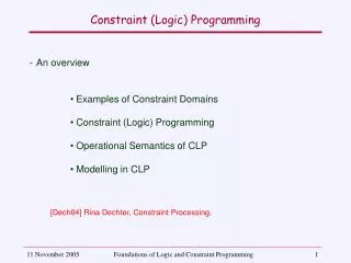
Constraint (Logic) Programming. An overview Examples of Constraint Domains Constraint (Logic) Programming Operational Semantics of CLP Modelling in CLP [Dech04] Rina Dechter, Constraint Processing,. Constraints and Constraint Problems.

Constraint (Logic) Programming
E N D
Presentation Transcript
Constraint (Logic) Programming • An overview • Examples of Constraint Domains • Constraint (Logic) Programming • Operational Semantics of CLP • Modelling in CLP [Dech04] Rina Dechter, Constraint Processing, Foundations of Logic and Constraint Programming
Constraints and Constraint Problems • Formally a constraint (solving) problem can be regarded as a tuple <V, D, C>, where • X = { X1, ... , Xn} is a set of variables • D = { D1, ... , Dn} is a set of domains (for the corresponding variables) • C = { C1, ... , Cm} is a set of constraints (on the variables) • Solving a constraint problem consists of determining values xi Difor each variable Xi, satisfying all the constraints C. • Intuitively, a constraint Ci is a limitation on the values of its variables. • More formally, a constraint Ci (with arity k) over variables Xi1, ..., Xik ranging over domains Di1, ..., Dik is a subset of the cartesian cartesian Dj1 ... Djk. Ci Dj1 ... Djk Foundations of Logic and Constraint Programming
Constraint Problems: Examples • Examples of these problems include • Modelling of Digital Circuits • Production Planning • Network Management • Scheduling (Qualitative and Quantitative) • Assignment (Colouring, Latin/ Magic Sqaures, Sudoku, Circuits, ...) • Assignment and Scheduling (Timetabling, Job-shop) • Filling and Containment • Scene Interpretation Foundations of Logic and Constraint Programming
E = or(A,B) % G1 F = nand(B,C) % G2 G = and(B,C) % G3 H = nand(E,F) % G4 I = nand(F,G) % G5 A E G1 G4 H B F G2 C G G5 I G3 D Modeling of Digital Circuits Goal (Example): Determine a test pattern that detects some faulty gate • Variables: • Signals in the circuit • Domain: • Booleans: 0/1 (or True/False, or High/Low) • Constraints: • Equality constraints between the output of a gate and its “boolean operation” (e.g. and, or, not, nand, ...) Foundations of Logic and Constraint Programming
Production Planning Goal (Example): Determine a production plan • Variables: • Quantities of goods to produce • Domain: • Rational/Reals or Integers • Constraints: • Equality and Inequality (linear) constraints to model resource limitations, minimal quantities to produce, costs not to exceed, balance conditions, etc... Find X, Y and Z such that 4x+ 3y + 6z 1500 % resources used do not exceed 1500 x + y + z >= 300 % production not less than 300 units x z + 20 % x units within z 20 units x z - 20 x, y, z 0 % non negative production Foundations of Logic and Constraint Programming
x 5/a Find x,y,z, a,b,c,d,e such that x 6, z 10 % minimum flow a 5, ... , f 6 % capacity % flow maintenance x = a, y = b + c, a + b + d = e, c = d + f, e + f = z x, y ,z, a, b, c, d, e, f 0 3/b y 8/e 2/d 7/c z 6/f Network Management Goal (Example): Determine acceptable traffic on a netwok • Variables: • Flows in each edge • Domain: • Rational/Reals (or Integers) • Constraints: • Equality and Inequality (linear) constraints to model capacity limitations, flow maintenance, costs, etc... Foundations of Logic and Constraint Programming
Tb Find Sa ,..., Se, such that Sb Sa+Ta, % precedence .... (Sc Sb+Tb)(Sb Sc+Tc)% non overlap ..., 6 Sa+Ta % deadline Sa,..., Se0 Ta Td Sa Sc Sb Se Sd Tc Ta Schedulling (Quantitative) Goal (Example): Assign timing/precedence to tasks • Variables: • Start Timing of Tasks, Duration of Tasks • Domain: • Rational/Reals or Integers • Constraints: • Precedence Constraints, Non-overlapping constraints, Deadlines, etc... Foundations of Logic and Constraint Programming
? What relation between C and D, given that A preceeds B, B preceeds C, C meets E A preceeds D, D meets E, B overlaps D A D B E C Schedulling (Qualitative) Goal (Example): Complete assignment of task relations • Variables: • Relations between tasks (qualitative; e.g Ta preceedes Tb) • Domain: • 16 relations (preceeds, meets, overlap, ....) • Constraints: • Partial assignments Foundations of Logic and Constraint Programming
Assignment Many constraint problems can be classified as assignment problems. In general all that can be stated is that these problems follow the general goal CSPs: Assign values to the variables to satisfy the relevant constraints. • Variables: • Objects / Properties of objects • Domain: • Integer, enumerated or Real Values (properties - colours, numbers, ..) • Booleans for decisions • Constraints: • Compatibility (Equality, Difference, No-attack, Arithmetic Relations) Some examples may help to illustrate this class of problems Foundations of Logic and Constraint Programming
Graph Colouring (Booleans) Assign values to A1,A2, .., F1,F2 s.t. A1,A2, .., F1,F2 {0,1} % different colours for A and B A1 B1 or A2 B2 .... E1 F1 or E2 F2 Graph Colouring (Finite Domains) Assign values to A, .., F, s.t. A, B, .., F {red, blue, green} A B, A C, A D, B C, B F, C D, C E, C F D E, E F B B A A C C D D F F E E Assignment (2) Foundations of Logic and Constraint Programming
N-queens (Finite Domains): Assign Values to Q1,..., Qn {1,.., n} s.t. ijnoattack (Qi, Qj) Latin Squares (similar to Sudoku): Assign Values to X11,..., X33 {1,.., 3} s.t. ijkXij Xik % same row jikXij Xkj % same column Magic Squares: Assign Values to X11,..., X33 {1,..,9} s.t. ijSk Xki= Xkj % same rows sum ij Sk Xik = Xjk % same cols sum ik jl Xij Xkl % all different Assignment (3) Foundations of Logic and Constraint Programming
Travelling Salesperson (Finite Domains) Find values for A, B, C, D {1,..,4} s.t. A B, ..., C D % a permutation of [A,B,C,D] if A = B+1then XA = Lab, ... if D = C+1 then XD = Lcd Xa + Xb + Xc + Xd K 23 23 A A B B 13 13 21 21 17 17 18 18 C C D D 33 33 Travelling Salesperson (Booleans) Find decision values for Xab...Xdc {0,1} s.t. a Sk Xak = 1 aSk Xka = 1 no subcycle constraints SaSb Xab Lab < k Assignment (3) Foundations of Logic and Constraint Programming
Mixed: Assignment and Scheduling Goal (Example): Assign values to variables • Variables: • Start Times, Durations, Resources used • Domain: • Integers (typicaly) or Rationals/Reals • Constraints: • Compatibility (Disjunctive, Difference, Arithmetic Relations) Job-Shop Assign values to Sij {1,..,n} % time slots and to Mij {1,..,m} % machines available % precedence within job j i < kSij + Dij ≤ Skj % either no-overlap or different machines i,j,k,l(Mij ≠Mkl)(Sij +Dij ≤Skl)(Skl +Dkl ≤Sij) Foundations of Logic and Constraint Programming
Filling and Containment Goal (Example): Assign values to variables • Variables: • Point Locations • Domain: • Integers (typicaly) or Rationals/Reals • Constraints: • Non-overlapping (Disjunctive, Inequality) Fiiling Assign values to Xi {1,.., Xmax} % X-dimension Yi {1,.., Ymax}% Y-dimension % no-overlapping rectangles i,j (Xi+Lxi Xj) % I to the left of J (Xj+Lxj Xi) % I to the right of J (Yi+Lyi Yj) % I in front of J (Yj+Lxj Xi) % I in back of J Foundations of Logic and Constraint Programming
Scene Interpretation Goal (Example): Assign values to junctions • Variables: • Junctions • Domain: • Junction Types • Constraints: • Compatibility of junctions Foundations of Logic and Constraint Programming
Constraint Programming Constraint Programming and Languages is driven by a number of goals • Expressivity • Constraint Languages should be able to easily specify the variables, domains and constraints (e.g. conditional, global, etc...); • Declarative Nature • Ideally, programs should specify the constraints to be solved, not the algorithms used to solve them • Efficiency • Solutions should be found as efficiently as possile, i.e. With the minimum possible use of resources (time and space). These goals are partially conficting goals and have led to the various developments in this research and development area. Foundations of Logic and Constraint Programming
Complexity of Constraint Problems Assuming that a potential solution can be generated and tested in 1 μs, the approximate times required to search the whole space of the kn possible solutions is given in the table This complexity is in sharp constrast with the complexity of deterministic problems (such as sorting of lists, matrix multiplication, etc, which are polinomial on the size n of the structures 1 hour = 3.6*103 ; 1 day = 8.6*104 ; 1 year =3.1*107 ; age of universe = 4.7*1023 Foundations of Logic and Constraint Programming
Complexity of Constraint Problems A major issue in constraint solving problems is their complexity. In general these are combinatorial problems with an exponential search space. • Booleans • Number of Variables: n • Domain cardinality: 2 • Number of potential solutions: 2n • Finite Domains • Number of Variables: n • Domain cardinality: d • Number of potential solutions: dn • Real/Rational Domains • Number of Variables: n • Domain cardinality: Theoretically infinite. In practice finite, D, due to rounding. • Number of potential solutions: Dn Foundations of Logic and Constraint Programming
Prob SAT Constraint Problems are NP • Notwithstanding the exponential number of the search space, one could expect that in practice solutions are found much quicker by some “cleaver” procedure. • Nevertheless, most decision problems of interest, (e.g. those described before) are NP–complete, i.e. they are of the same complexity of the Satisfiability problem for Boolean Clauses (SAT). • This equivalence of SAT and a problem Prob is proven in general by the transformation (in polinomial time) of SAT into Prob, and of Prob into SAT. • Given this equivalence, if there was a procedure to solve SAT in polinomial time, all NP problems would be solved in polinomial time as well. • Unfortunately, no one has ever found such procedure in general. For a given procedure, it has always been possible to find instances of SAT that are solved in exponential time. Foundations of Logic and Constraint Programming
Constraint Problems are NP • Notice that the NP nature of these decision problems does not prevent that for many problem instances it is possible to find efficient procedures to solve them. • In practice, a problem is NP-complete if it is possible to check a solution in polinomial time (to find a solution may take exponential time). • Decision problems lie in this category, since given some potential solution one has only to check one by one, all the constraints (a number usually in the order of magnitude of the variables). • Optimisation problems are usually harder than decision ones, hence their classification as NP-Hard. • Here checking a solution usually requires exponential time, since it requires to compare all solutions (and hence find them, which requires exponential time). Foundations of Logic and Constraint Programming
Declarative Programming • Programming a combinatorial problem requires • the specification of the constraints of the problem • The specification of a search algorithm • The separation of these two aspects has for a long time been advocated by several programming paradigms, namely functional programming and logic programming.. • Logic programming in particular has a built in mechanism for search (backtracking) that makes it a good candidate to constraint programming. • Maintaining its search mechanism, all that is required is to extend its underlying resolution to constraint solving. • This is in fact quite natural, since resolution may be regarded as a particular type of constraint solving, namely the equality of Herbrand terms (trees), which is performed in the unification of a goal and a clause head. Foundations of Logic and Constraint Programming
Operational Semantics of CLP • The operational semantics of Constraint Logic Programming can be described as a transition system on states. • The state of a constraint solving system can be abstracted by a tuple < G, CS > where • G is a set of constraints still to solve • CS is the Constraint Store: a set of constraints already examined • In LP, G is the query, i.e. the set of goals still to solve. Set CS maintains the composition of all the unifications performed in the previous resolution steps. • A derivation is just a sequence of transitions. • A state that cannot be rewritten is a final state. • An executor of (C)LP aims at finding successful final states of derivations starting with a query. Foundations of Logic and Constraint Programming
g requires solving c and other goals G’ < G {g}, CS >s < G G’, CS {c} > State Transitions of CLP • A derivation is failed if it is finite and its final state is fail. • A derivation is successful if it is finite and processes all the constraints, i.e. it ends in a state with form <Ø, S > • The state transitions are the following S(elect): Select a goal (constraint) • It is assumed that • A computation rule selects some goal g, among those still to be considered that requires solving of some constraint c. • The set of unsolved goals is eventually augmented with set G’, with additional goals to be further considered. Foundations of Logic and Constraint Programming
CS’ = infer(CS {c}) < G, CS {c})>i < G, CS’> consistent (CS) ¬consistent (CS) < G, CS >c < G, CS > < G, CS>c fail State Transitions of CLP • The other transition rules require the existence of two functions, infer(C,S) and consistent(C), adequate to the domains that are considered. • I(nfer): Process a constraint, inferring its consequences • C(heck): Check the consistency of the Store Foundations of Logic and Constraint Programming
g is a goal h B < G {g}, CS >s < G B, CS {h = g} > State Transitions of LP In Logic Programming • Handling a goal g is simply checking whether there is a clause H ← B whose head h matches the goal. In this case, the equality constraint between Herbrand terms g=h is added to the passive store. • Function infer(C,c) performs unification of the terms included in g and h, after applying all substitutions included in C function infer(q, g=h) if unify(g q,h q, s) then infer = (success, s) else infer = (fail,_); end function • Checking consistency is a simple check on whether the previous unification has returned success or failure (in practice the two functions are merged). Foundations of Logic and Constraint Programming
State Transitions of LP: Example • For example, assuming that • CS = {X / f(Z), Y / g(Z,W)} % a solved form • G includes goal p(Z,W) • there is a clause p(a,b) :- B. then the following transitions take place, when goal p(Z,W) is “called” < G , {X/f(Z), Y/g(Z,W)} > →s % goal selection < G \ {g} B, {X/f(Z), Y/g(Z,W)} {p(Z,W) = p(a,b)}} > →i,c % unification (inference and consistency check) < G \ {g} B, {X/f(a), Y/g(a,b), Z/a, W/b} > Foundations of Logic and Constraint Programming
g is a constraint < G {g}, CS >s < G, CS {g} > State Transitions of CLP In Constraint Logic Programming • Handling a goal g is as before. Handling a constraint in a certain domain, usually built-in, simply places the constraint in set CS. . • Function infer(C,S) propagates the constraint in the Constraint Store, by methods that depend on the constraint system used. Tipically, • It attempts to reduce the values in the domains of the variables; or • obtain a new solved form (like in unification) • Checking consistency also depends on the constraint system. • It checks whether a domain has become empty; or • Whether it was not possible to obtain a solved form. Foundations of Logic and Constraint Programming
State Transitions of CLP: Example (1) A positive example • Assuming that variables A and B can take values in 1..3, then the constraint store may be represented as CS = {A in 1..3, B in 1..3} • Rule S: If the constraint selected by rule S is A > B, then the store becomes CS = {A in 1..3, B in 1..3} {A > B} • Rule I: The Infer rule propagates this constraint in the constraint store, which becomes C,S = {A in 2..3, B in 1..2, A > B} • Rule C: The system does not find any inconsitency in the active store, so the system does not change. Foundations of Logic and Constraint Programming
State Transitions of CLP: Example (2) A negative example • Assuming that variables A and B can take, respectively values in the sets {1,3,5} and {2,4,6}. The constraint store may be represented as CS = { A in {1,3,5} B in {2,4,6} } • Rule S: If the constraint selected by rule S is A = B, the store becomes CS = { A in {1,3,5} B in {2,4,6} } { A = B } • Rule I: The rule propagates this constraint to the active store. Since no values are common to A and B, their domains become empty CS = {A in {}, B in {} } • Rule C: This rule finds the empty domains and makes the transition to fail (signaling the system to backtrack in order to find alternative successful derivations). Foundations of Logic and Constraint Programming
Solutions in (C)LP • In LP and CLP, solutions are obtained, by inspecting the constraint store of the final state of a successful derivation. • In systems that maintain a solved form, (like LP, but also constraint systems CLP(B) for booleans, and CLP(Q), for rationals), solutions are obtained by projection of the store to the relevant variables. For example if the initial goal was p(X,Y) and the final store is {X/f(Z,a), Y/g(a,b), W/c} then the solution is the projection to variables X and Y {X/f(Z,a), Y/g(a,b), W/c} • In systems where a solved form is not maintained, solutions require some form of enumeration. For example, from C = {X in 2..3, Y in 1..2, X > Y}, the solutions <X=2;Y=1>, <X=3;Y=1> and <X=3;Y=1>, are obtained by enumeration. Foundations of Logic and Constraint Programming
The CLP approach to Constraint Solving • To program a constraint solving problem in CLP a number of issues must be taken into account • What is the purpose of the program? • Any (first) solution? • All solutions ? (decision making with uncertainty) • Best Solution? (optimisation) • What kind of modeling? • Variables and Domains? (Finite Domains? Booleans? Sets? Mixed?) • Constraints ? (Global? Redundant? ) • What solver should be used? • Complete Solver? (All solutions, inneficiency?) • Incomplete solvers ? (Single solutions, Heuristics?) • An example, N-queens, will illustrate some of these issues. Foundations of Logic and Constraint Programming
N-Queens • The N-queens problem consists of finding positions for N queens in a NN chess-board, so that no 2 queens attack each other. • Modeling: • Boolean Variables: One 0/1 variable for each position of the board • SAT or arithmetic constraints ? • Finite Domains: One 1..N variable for each row in the board • Solvers: • Complete (only for Booleans): • maintains all solutions • Incomplete: Booleans / Finite Domains: • One solution at a time • In this case there is no clear optimisation purpose (function to optimise) Foundations of Logic and Constraint Programming
N-Queens Models • Assuming Boolean variables, Xij (i,j 1..n), one per position • Constraints • One per Row (One per column is similar) • SAT: Xij \/ ...\/ Xinfor all i 1..n • Xij \/ Xikfor all i, j k 1..n • Arithmetic: Xij + ...+ Xin = 1 for all i 1..n • Diagonals • SAT: Xij \/ Xklfor all i+j = k+l and all i-j = k-l • Arithmetic: Sij Xij 1 for all ij = k -2n-1 .. 2n+1 • Assuming Finite Domain variables, Xi (i 1..n), ), one per row • Constraints (one per row is implicit) • One per Column Xi Xjfor all i j 1..n • Diagonals: Xi Xj for all i+j = k -2n-1 .. 2n+1 Foundations of Logic and Constraint Programming
CLP Programs • CLP programs have in general the following structure Program • Variable Declaration % not needed in complete solvers • Constraint Declaration • Search % optional in all solutions/complete solvers • In general, CLP systems require the addition of modules that implement the intended solvers. For example in SICStus :- use_module(library(clpb)). the complete solver for booleans :- use_module(library(clpfd)). The solver for finite domains • Such solvers identify constraints and goals with a different syntax • sat(X+Y =:= 1) implements an “OR” of boolean variables X and Y • X+Y #= 3 enforces the sum of FD variables X and Y to be 3 • In the rest, CLP programs adopt the syntax of LP (Prolog) Foundations of Logic and Constraint Programming
Boolean N-Queens: Complete Solver • For simplicity, we show the 3-queens program. It can be easily adapted for larger boards (3-queens has no solutions). :- clpb. queens_3(Q):- Q = [Q11, Q12, Q13, Q21, Q22, Q23, Q31, Q32, Q33], % one and only one queen per row sat(Q11+Q12+Q13 =:= 1),sat(Q11*Q12=:=0),sat(Q11*Q13=:=0),sat(Q12*Q13=:=0), sat(Q21+Q22+Q23 =:= 1),sat(Q21*Q22=:=0),sat(Q21*Q23=:=0),sat(Q22*Q23=:=0), sat(Q31+Q32+Q33 =:= 1),sat(Q31*Q32=:=0),sat(Q31*Q33=:=0),sat(Q32*Q33=:=0), % one and only one queen per column sat(Q11+Q21+Q31 =:= 1),sat(Q11*Q21=:=0),sat(Q11*Q31=:=0),sat(Q21*Q31=:=0), sat(Q12+Q22+Q32 =:= 1),sat(Q12*Q22=:=0),sat(Q12*Q32=:=0),sat(Q22*Q32=:=0), sat(Q13+Q23+Q33 =:= 1),sat(Q13*Q23=:=0),sat(Q13*Q33=:=0),sat(Q23*Q33=:=0), % no two queens in \ diagonals sat(Q11*Q22=:=0),sat(Q11*Q33=:=0),sat(Q22*Q32=:=0), sat(Q12*Q23=:=0),sat(Q21*Q32=:=0), % no two queens in \ diagonals sat(Q13*Q22=:=0),sat(Q13*Q31=:=0),sat(Q22*Q31=:=0), sat(Q12*Q21=:=0),sat(Q23*Q32=:=0). Foundations of Logic and Constraint Programming
Boolean N-Queens: SAT Solver :- op(300,fy,~). :- op(400,xfy,\/). :- clpfd. queens_3(Q):- % variable declaration Q = [Q11, Q12, Q13, Q21, Q22, Q23, Q31, Q32, Q33], domain(Q,0,1), % one and only one queen per row Q11 \/ Q12\/ Q13, ~Q11 \/ ~Q12, ~Q11 \/ ~Q13, ~Q12 \/ ~Q13, Q21 \/ Q22\/ Q23, ~Q21 \/ ~Q22, ~Q21 \/ ~Q23, ~Q22 \/ ~Q23, Q31 \/ Q32\/ Q33, ~Q31 \/ ~Q32, ~Q31 \/ ~Q33, ~Q32 \/ ~Q33, % one and only one queen per column Q11 \/ Q21\/ Q31, ~Q11 \/ ~Q21, ~Q11 \/ ~Q31, ~Q21 \/ ~Q31, Q12 \/ Q22\/ Q32, ~Q12 \/ ~Q22, ~Q12 \/ ~Q32, ~Q22 \/ ~Q32, Q13 \/ Q23\/ Q33, ~Q13 \/ ~Q23, ~Q13 \/ ~Q33, ~Q23 \/ ~Q33, % no two queens in \ diagonals ~Q11 \/ ~Q22, ~Q11 \/ ~Q33, ~Q22 \/ ~Q33, ~Q12 \/ ~Q23, ~Q21 \/ ~Q32, % no two queens in / diagonals ~Q13 \/ ~Q22, ~Q13 \/ ~Q31, ~Q22 \/ ~Q31, ~Q12 \/ ~Q21, ~Q23 \/ ~Q32, % enumeration (search) labeling([], Q). • The 3-queens program in SAT is shown with user-defined operators (“\/” and “~”), implemented in the FD solver. Foundations of Logic and Constraint Programming
Boolean N-Queens: Arithmetic Solver :- op(300,fy,~). :- op(400,xfy,\/). :- clpfd. queens_3(Q):- % variable declaration Q = [Q11, Q12, Q13, Q21, Q22, Q23, Q31, Q32, Q33], domain(Q,0,1), % one and only one queen per row Q11 + Q12 + Q13 #= 1, Q21 + Q22 + Q23 #= 1, Q31 + Q32 + Q33 #= 1, % one and only one queen per column Q11 + Q21 + Q31 #= 1, Q12 + Q22 + Q32 #= 1, Q13 + Q23 + Q33 #= 1, % no two queens in \ diagonals Q11+Q21 #=<1, Q11+Q33 #=<1, Q22+Q33 #=<1, Q12+Q23 #=<1, Q21+Q32 #=<1, % no two queens in / diagonals Q13+Q22 #=<1, Q13+Q31 #=<1, Q22+Q31 #=<1, Q12+Q21 #=<1, Q23+Q32 #=<1, % enumeration (search) labeling([], Q). • The 3-queens program with boolean variables may be more easily expressed with arithmetic constraints. Foundations of Logic and Constraint Programming
Finite Domains N-Queens • The 3-queens program in FD is much simpler, since with much less variables. :- clpfd. queens_3(Q):- % declaration of variables Q = [Q1,Q2,Q3], % only one queen in each row domain(Q,1,3), % one and only queen in each column Q1 #\= Q2, Q2 #\=Q3, Q1 #\= Q3, % no two queens in \ diagonals Q1+1 #\= Q2+2, Q1+1 #\= Q3+3, Q2+2 #\= Q3+3, % no two queens in / diagonals Q1-1 #\= Q2-2, Q1-1 #\= Q3-3, Q2-2 #\= Q3-3, % enumeration (search) labeling([],Q). Foundations of Logic and Constraint Programming
Finite Domains N-Queens • Of course, all these problems may be generalised for an arbitrary. size of the board, using all the constructs of Prolog, namely lists. This is the case with the FD model, shown below. compatible(_,[]). compatible(Past,[L-C|Future]):- compatible_1(L-C,Future), compatible([L-C|Past], Future). compatible_1(_,[]). compatible_1(L1-C1,[L2-C2|T]):- no_atack(L1,C1,L2,C2), compatible_1(L1-C1,T). no_atack(L1,C1,L2,C2):- C1 #\= C2, L1 + C1 #\= L2 + C2, L1 + C2 #\= L2 + C1. enumerate(Future):- clean(Future,L), labeling([ff],L). clean([],[]). clean([_-C|T1],[C|T]):- clean(T1,T). :-clpfd. queens_fd(N,Future):- create_vars(N,Future-[]), domainQ(N,Future), compatible([],Future), enumerate(Futuras). create_vars(0,Z-Z):- !. create_vars(N,L-Z):- M is N-1, create_vars(M,L-[N-_|Z]). domainQ(_,[]). domainQ(N,[_-C|Variables]):- C in 1 .. N, domainQ(N,Variables). Foundations of Logic and Constraint Programming