Projections and clipping in 3D
Viewing and projection. Objects in WC are projected on to the view plane, which is defined perpendicular to the viewing direction along the zv-axis. The two main types of projection in Computer Graphics are:parallel projectionperspective projection . Projection illustrations. Parallel projectionA

Projections and clipping in 3D
E N D
Presentation Transcript
1. Projections and clipping in 3D
2. Viewing and projection Objects in WC are projected on to the view plane, which is defined perpendicular to the viewing direction along the zv-axis. The two main types of projection in Computer Graphics are:
parallel projection
perspective projection
3. Projection illustrations Parallel projection
All projection lines are crossing the view plane in parallel; preserve relative proportions
Perspective projection
Projection lines are crossing the view plane and converge in a projection reference point (PRP)
4. Overview of projections
5. Parallel projection Two different types are used:
Orthographic (axonometric,isometric)
most common
projection perpendicular to view plane
Oblique (cabinet and cavalier)
projection not perpendicular to view plane
less common
6. Orthographic projection Assume view plane at zvp (perpendicular to the zv-axis) and (xv,yv,zv) an arbitrary point in VC
Then xp = xv
yp = yv
zp = zvp (zv is kept for depth purposes only)
7. Oblique projection When the projection path is not perpendicular to the view plane.
A vector direction is defining the projection lines
Can improve the view of an object
8. Oblique projection, cont�d An oblique parallel projection is often specified with two angles, ? (0-90�) och ? (0-360�), as shown below
9. Oblique formula (from fig.) Assume (x,y,z) any point in VC (cp. xv,yv,zv)
cos ?=(xp-x)/L => xp=x+L.cos ?
sin ??=(yp-y)/L => yp=y+L. sin ?
Also tan ?=(zvp-z)/L, thus L=(zvp-z)/tan ?= =L1(zvp-z), where L1=cot ?
Hence
xp = x + L1(zvp - z).cos ?
yp = y + L1(zvp - z).sin ?
Observe: if orthographic projection, then L1=0
10. Cavalier and Cabinet When
tan ? = 1 then the projection is called Cavalier (? = 45�)
tan ? = 2 then the projection is called Cabinet (? � 63�)
? usually takes the value 30� or 45�
11. Cavalier, example
12. Perspective projection
13. A general approach
14. Special cases Various restrictions are often used, such as:
PRP on the zv-axis (used in the next approach) => xprp=yprp=0
PRP in the VC origin => xprp=yprp=zprp=0
view plane in the xvyv-plane => zvp=0
view plane in the xvyv-plane and PRP on the zv-axis =>xprp=yprp=zvp=0
15. Special case: PRP on the zv-axis
16. Window and clipping in 3D
17. Window in 3D => View Volume A rectangular window on the view plane corresponds to a view volume of type:
infinite parallelepiped (parallel projection)
�half-infinite� pyramid with apex at PRP (perspective projection)
18. View volumes
19. Finite view volumes To get a finite volume (one or) two extra zv-boundary planes, parallel to the view plane, are added: the front (near) plane and the back (far) plane resulting in:
a rectangular parallelepiped (parallel projection)
a pyramidal frustum (perspective projection)
20. Finite view volumes
21. �Camera� properties The two new planes are mainly used as far and near clipping planes to eliminate objects close to and far from PRP (cp. the camera)
Other camera similarities:
PRP close to the view plane => �wide angle� lens
PRP far from the view plane => �tele photo� lens
Matrix representations for both parallel and per-spective projections are possible (see text book)
22. 3D Clipping A 3D algorithm for clipping identifies and saves those surface parts that are within the view volume
Extended 2D algorithms are well suited also in 3D; instead of clipping against straight boundary edges, clipping in 3D is against boundary planes, i.e. testing lines/surfaces against plane equations
23. Clipping planes Testing a point against the front and back clipping planes are easy; only the z-coordinate has to be checked
Testing against the other view volume sides are more complex when perspective projection (pyramid), but still easy when parallel projection, since the clipping sides are then parallel to the x- and y-axes
24. Clipping when perspective projection Before clipping, convert the view volume, a pyramidal frustum, to a rectangular parallelepiped (see next figure)
Clipping can then be performed as in the case of parallel projection, which means much less processing
From now on, all view volumes are assumed to be rectangular parallelepipeds (either including the special transformation or not)
25. The perspective transformation The perspective transformation will transform the object A to A� so that the parallel projection of A� will be identical to the perspective projection of A
26. Normalized coordinates A possible (and usual!) further transformation is to a unit cube; a normalized coordinate system (NC) is then introduced, with either 0=x,y,z=1 or -1=x,y,z=1
Since screen coordinates are often specified in a left-handed reference system, also normalized coordinates are often specified in a left-handed system, which means, for instance, viewing in the positive z-direction
27. Left-handed screen coordinates
28. Parallel projection view volume to normalized view volume
29. Perspective projection view volume to normalized view volume
30. Advantages with the parallelepiped/unit cube all view volumes have a standard shape and corresponds to common output devices
simplified and standardized clipping
depth determinations are simplified when it comes to Visible Surface Detection
31. Clipping in more detail Both the 2D algorithms, Cohen-Sutherland�s for line clipping and Sutherland-Hodgeman�s for polygon clipping, can easily be modified to 3D clipping.
One of the main differences is that clipping has to be performed against boundary planes instead of boundary edges
Another is that clipping in 3D generally needs to be done in homogeneous coordinates
32. Clipping details,cont�d With matrix representation of the viewing and projection transformations, the matrix M below represent the concatenation of all various transformations from world coordinates to normalized, homogeneous projection coordinates with h taking any real value!
33. Line clipping
34. Polygon clipping Graphics packages typically deal only with objects made up by polygons
Clipping an object is then broken down in clipping polygon surfaces
First, some bounding surface is tested
Then, vertex lists as in 2D but now processed by 6 clippers!
Additional surfaces need to �close� cut objects along the view volume boundary
Concave objects are often split
35. Example, object clipping
36. Viewing pipeline After the clipping routines have been applied to the normalized view volume, the remaining tasks are:
Visibility determination
Surface rendering
Transformation to the viewport (device)