Basic Macroeconomic Relationships
Basic Macroeconomic Relationships. Chapter 9. Chapter 9 Figure 9.1. Average Propensities APC = C/DI APS = S/DI since DI = S + C APC + APS = 1. Marginal Propensities MPC = ∆C/∆DI MPS = ∆S/∆DI Since DI = S + C ∆DI = ∆S + ∆C MPC + MPS = 1.


Basic Macroeconomic Relationships
E N D
Presentation Transcript
Basic Macroeconomic Relationships Chapter 9
Average Propensities APC = C/DI APS = S/DI since DI = S + C APC + APS = 1 Marginal Propensities MPC = ∆C/∆DI MPS = ∆S/∆DI Since DI = S + C ∆DI = ∆S + ∆C MPC + MPS = 1 Average and Marginal Propensities to Consume and Save
Chapter 9 Figure 9.2 The Consumption and Saving Functions
Consumption and Saving Functions I • Consumption function: • C = CA + MPC(Y) • Where • CA (intercept) = “Autonomous Consumption” • MPC (slope) = “Marginal Propensity to Consume” (also = 1 – MPS) • Y = GDP or “Disposable Income”
Consumption and Saving Functions II • Saving function: • S = S0 + MPS(Y) • Where • S0 (intercept) = “Maximum Dissaving” = - CA • MPS (slope) = “Marginal Propensity to Save” (also = 1 – MPC) • Y = GDP or “Disposable Income”
Consumption and Saving Functions III • Since CA = - S0 and MPS +MPC = 1 • If the consumption function is • C = 100 + .85Y • The saving function must be • S = -100 + .15Y • If the saving function is • S = -125 + .3Y • The consumption function must be • C = 125 + .7Y
Chapter 9 Figure 9.4(a) Shifting the Consumption Schedule
Chapter 9 Figure 9.4(b) Shifting the Saving Schedule
Chapter 9 Table 9.2 The Investment Demand Schedule
Chapter 9 Figure 9.5 The Investment Demand Function
What Shifts the Investment Demand Function? • Changes in the cost of acquiring capital equipment, maintaining capital equipment, or operating capital equipment • e.g., changes in the price of gasoline • Changes in taxes on business • e.g., accelerated depreciation • Technological Improvements • How much capital equipment is already installed • Producer Expectations • Overoptimistic during the expansionary phase of the business cycle • Frustrating efforts to slow down the economy • Overpessimistic during the contractionary phase of the business cycle • Delaying recovery
Chapter 9 Figure 9.7 Investment is highly volatile!
Chapter 9 Table 9.3 The AE multiplier M = 1/(1- MPC) = 1/MPS
The Multiplier Formula • First round, increase in Aggregate Expenditure = ∆AE0 • This induces an increase in C, ∆C1 = (MPC)∆AE0 • Which becomes the second round increase in income • Inducing a further increase in C, ∆C2 = (MPC)∆C1 = (MPC)2∆AE0 • ∆C3 = (MPC)∆C2 = (MPC)3∆AE0, etc.
Derivation of the Multiplier • ∆Y = ∆AE0 + ∆AE1 + ∆AE2 + ∆AE3 + … + ∆AEn + … • ∆Y = ∆AE0 + (MPC)∆AE0 + (MPC)∆AE1 + (MPC)∆AE2 + … + ∆AEn + … • ∆Y = ∆AE0 + (MPC)∆AE0 + (MPC)2∆AE0 + (MPC)3∆AE0 + … + (MPC)n∆AE0 + … • ∆Y = (MPC)0∆AE0 + (MPC)1∆AE0 + (MPC)2∆AE0 + (MPC)3∆AE0 + … + (MPC)n∆AE0 + …
Derivation of the Multiplier • ∆Y = (MPC)0∆AE0 + (MPC)1∆AE0 + (MPC)2∆AE0 + (MPC)3∆AE0 + … + (MPC)n∆AE0 + … • ∆Y = ∑i=0,∞(MPC)n∆AE0 = ∆AE0∑i=0,∞(MPC)n • for infinite convergent sums, • m = ∆Y/∆AE = 1/(1 – MPC) = 1/MPS • MPC < 1 necessary for infinite sum to converge
Chapter 9 Figure 9.9 How M varies with the MPC
The AE multiplier • M = 1/(1- MPC) = 1/MPS • M = change in real GDP/change in spending • M = ∆GDP/∆AE = ∆Y/∆AE • Change in AE can come from any component of aggregate expenditure • AE = C + Ig + G + Xn