Download
1 / 16
190 likes | 439 Vues
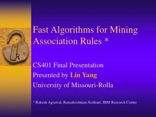
Fast Algorithms for Mining Association Rules *. CS401 Final Presentation Presented by Lin Yang University of Missouri-Rolla * Rakesh Agrawal, Ramakrishnam Scrikant, IBM Research Center. Outlines. Problem: Mining association rules between items in a large database

E N D
Fast Algorithms for Mining Association Rules * CS401 Final Presentation Presented by Lin Yang University of Missouri-Rolla * Rakesh Agrawal, Ramakrishnam Scrikant, IBM Research Center
Outlines • Problem: Mining association rules between items in a large database • Solution: Two new algorithms • Apriori • AprioriTid • Examples • Comparison with other algorithms(SETM &AIS) • Conclusions
Introduction • Mining association rules: Given a set of transactions D, the problem of mining association rules is to generate all association rules that have support and confidence greater than the user-specified minimum support(called minsup) and minimum confidence(called minconf) respectively
Example:98% of customer who buy bread also buy milk. Bread means or implies milk 98% of the time. Terms and Concepts • Associations rules,Support and Confidence Let L={i1,i2,….im} be a set of items. Let D be a set of transactions, where each transaction T is a set of items such that TL An association rule is an implication of the form X=>Y, where XL,Y L, and XY=. The rule X=>Y holds in the transactions set D with confidence c if c% of transaction in D that contain X also contains Y. The rule X=>Y has support s in the transaction set D if s% of transaction in D contain XY
Problem Decomposition • Find all sets of items that have transaction support above minimum support. The support for an itemset is the number of transactions that contain the itemset. Itemsets with minimum support are called large itemsets • Use the large itemsets to generate the desired rules.
Discover Large Itemsets • Step 1: Make multiple passes over the data and determine large itemsets, i.e. with minimum support • Step 2: Use seed set for generating candidate itemsets and count the actual support • Step 3: determine the large candidate itemsets and use them for the next pass • Continues until no new large itemsets are found
Set of large k-itemsets(those with minimum support)Each member of this set has two fields i)itemset ii)support count Set of candidate k-itemsets(potentially large itemsets).Each member of this set has two fields: i)itemset and ii) support count Algorithm Apriori 1) L1 = large 1-itemsets; 2) for (k=2; Lk-10; k++) do begin 3) Ck = aprioti-gen(Lk-1); // New candidates 4) for all transactions tD do begin 5) Ct=subset(Ck, t); // Candidate contained in t 6) for all candidates c Ct do 7) c.count++; 8) end; 9) Lk = {c Ck | c.count minsup}; 10) end; 11) Answer = kLk;
Apriori Candidate Generation • Insert into Ck select p.item1, p.item2, …p.itemk-1,q.itemk-1 from Lk-1p, Lk-1q where p.item1=q.item1,…. p.itemk-2=q.itemk-2 p.itemk-1<q.itemk-1 next ,in the prune stepwe delete all itemsets cCk such that some (k-1) –subset of c is not in Lk-1: for all itemsets set cCk do for all (k-1) –subset s of c do if ( sLk-1) then delete c form Ck
An Example of Apriori L1={1,2,3,4,5,6} Then the candidate set that will be generated by our algorithm will be: C2={{1,2}{1,3}{1,4}{1,5}{1,6}{2,3}{2,4}{2,5} {2,6}{3,4}{3,5}{3,6}{4,5}{4,6}{5,6}}Then from the candidate set we generate the large itemset L2={{1,2},{1,3},{1,4},{1,5},{2,3},{2,4},{3,4},{3,5}} whose support =2 C3={{1,2,3},{1,2,4},{1,2,5}{1,3,4},{1,3,5},{1,4,5}{2,3,4},{3,4,5}}Then from the candidate set we generate the large itemset Then the prune step will delete the itemset {1,2,5}
An Example of Apriori {1,4,5} {3,4,5} because {2,5}{4,5} are not in L2 L3={{1,2,3},{1,2,4},{1,3,4},{1,3,5},{2,3,4}} suppose All of these itemsets has support not less than 2 C4 will be {{1,2,3,4}{1,3,4,5}} the prune step will delete the itemset {1,3,4,5} because the itemset {1,4,5} is not it L3 we will then be left with only {1,2,3,4} in C4 L4={} if the support of {1,2,3,4} is less than 2. And the algorithm will stop generating the large itemsets.
Advantages • The Apriori algorithm generates the candidate itemsets found in a pass by using only the itemsets found large in the previous pass – without considering the transactions in the database. The basic intuition is that any subset of a large itemset must be large. Therefore, the candidate itemsets having k items can be generated by joining large itemsets having k-1 items, and deleting those that contain any subset that is not large. This procedure results in generation of a much smaller number of candidate itemsets.
Set of candidate k-itemsets when the TIDs of the generating transactions are kept associated with the candidates (TID: the unique identifier Associated with each transaction Algorithm AprioriTid • ApriotiTid algorithm also uses the apriori-gen function to determine the candidate itemsets before the pass begins. The interesting feature of this algorithm is that the database D is not used for counting support after the first pass. Rather, the set Ck’ is used for this purpose.
Average size of the transactions • Number of Transactions • Average size of the maximal potentially large itemsets Comparison with other algorithms • Parameter Settings
Diagram 1-6 show the execution times for the six datasets given in the table on last slide for decreasing values of minimum support. As the minimum support decreases, the execution times of all the algorithms increase because of increases in the total number of candidate and large itemsets. For SETM, we have only plotted the execution times for the dataset T5.I2.D100K in Relative Performance (1). The execution times for SETM for the two datasets with an average transaction size of 10 are given in Performance (7). For small problems, AprioriTid did about as well as Apriori, but performance degraded to about twice as slow for large problems. Apriori beat AIS for all problem sizes, by factors ranging from 2 for high minimum support to more than an order of magnitude for low levels of support. AIS always did considerably better than SETM. Relative Performance (1-6) For the three datasets with transaction sizes of 20, SETM took too long to execute and we aborted those runs as the trends were clear. Clearly, Apriori beats SETM by more than an order of magnitude for large datasets.
We did not plot the execution times in Performance (7) on the corresponding graphs because they are too large compared to the execution times of the other algorithms. Relative Performance (7) Clearly, Apriori beats SETM by more than an order of magnitude for large datasets.
Conclusion • We presented two new algorithms, Apriori and AprioriTid, for discovering all significant association rules between items in a large database of transactions. We compared these algorithms to the previously known algorithms, the AIS and SETM. We presented the experimental results, showing that the proposed algorithms always outperform AIS and SETM. The performance gap increased with the problem size, and ranged from a factor of three for small problems to more than an order of magnitude for large problems.