Download
1 / 33
340 likes | 507 Vues
An introduction to the physics of the interstellar medium III. Hydrodynamics in the ISM. Patrick Hennebelle. The Equations of Hydrodynamics. Equation of state:

E N D
An introduction to the physics of the interstellar medium III. Hydrodynamics in the ISM Patrick Hennebelle
The Equations of Hydrodynamics Equation of state: Continuity Equation: consider a layer of gas of surface S between x and x+dx -the incoming flux is rv(x) while the flux leaving the layer is rv(x+dx) -the variation of mass between time t and t+dt is r(t+dt)-r(t) -as mass is concerned: (r(t+dt)-r(t)) S dx = (rv(x)-rv(x+dx)) S dt Momentum Conservation: Consider a fluid particle of size dx (surface S), on velocity v. During t and t+dt the linear momentum variation is due to the external forces (say only pressure to simplify) S dx ( v(t+dt)-v(t) ) = P(x) S – P(x+dx) S dt => Heat Equation: -second principe of thermodynamics: dU = TdS – PdV, U=kb/mp(g-1) -assume no entropy creation (heat created by dissipation and no entropy exchanged) -dV=-dr/r2 => dU=Pdr/r2 => rdU/dt = -Pdiv(v) =>
A simple Application: Sound Waves Consider a linear pertubation in a plan-parallel uniform medium: We linearize the equations: Continuity equation Conservation of momentum Combining these two relations we obtain the dispersion relation:
A less simple Application: Thermal Instability Consider a linear pertubation in a plan-parallel uniform medium: We linearize the equations: Continuity equation Conservation of momentum Perfect gas law Energy conservation Combining these two relations we obtain the dispersion relation: Field 1965
Existence of 3 different modes: -isochoric: essentially temperature variation -isentropic: instability of a travelling sound waves -isobaric: corresponds to a density fluctuations at constant pressure The latter is usually emphasized -At large wave number the growth rate saturates and becomes independent of k -At small wave number it decreases with k -the growth rate decreases when the conductivity increases as it transports heats and tends to erase temperature gradients Growth rate Field 1965 Wave number
Structure of Thermal Fronts (Zeldowich & Pikelner 1969) Question: what is the “equilibrium state” of thermal instability ? r lf CNM - - + + WNM X The CNM and the WNM are at thermal equilibrium but not the front between them. Equilibrium between thermal balance and thermal conduction which transports the heat flux. The typical front length is about: . It is called the Field length. In the WNM this length is about 0.1 pc while it is about 10-3 pc in the CNM
Propagation of Thermal Fronts The diffuse part of the front heats while the dense part cools =>in general the net balance is either positive or negative =>conversion of WNM into CNM or of CNM into WNM =>Clouds evaporate or condense The flux of mass is given by: There is a pressure, Ps, such that J=0 when heating=cooling If the pressure is higher than Ps the front cools and the cloud condenses If the pressure is lower than Ps the front heats and the cloud evaporates The 2-phase structure leads to pressure regulation and is likely to fix the ISM pressure! If the pressure becomes too high WNM->CNM and the pressure decreases while if it becomes low CNM->WNM.
Big powerlaws in the sky….. Turbulence ? Density of electrons within WIM (Rickett et al. 1995) Intensity of HI and dust emission Gibson 2007
A brief and Phenomenological Introduction to incompressible Turbulence Turbulence is by essence a multi-scale process which entails eddies at all size. Let us again have a look to the Navier-Stokes equation. Dissipation term. Converts mechanical energy into thermal energy => Stops the cascade Linear term. Involved in the sound wave propagation Non-linear term. Not involved in the sound wave propagation =>couples the various modes creating higher frequency modes =>induces the turbulent cascade The Reynolds number describes the ratio of the non-linear advection term over the dissipative term: Low Reynolds number: flow is very viscous and laminar High Reynolds number: flow is “usually” fully turbulent
Let us consider a piece of fluid of size, l, the Reynolds number depends on the scale Thus, on large scales the flow is almost inviscid, energy is transmitted to smaller scales without being dissipated while there is a scale at which the Reynolds number becomes equal to 1 and energy is dissipated. This leads to the Richardson Cascade: Injection of Energy at large scales Flux of Energy at intermediate scales Dissipation of Energy at small scales
Let us consider the largest scale L0 and the velocity dispersion V0. A fluid particle crosses the system in a turnover time: t0=L0/V0. The specific energy V02 cascades in a time of the order of t0. Let us define equal to the flux of energy injected in the system. In the stationary regime, this energy has to be dissipated and must therefore be transferred toward smaller scales through the cascade. Kolmogorov assumption is that: at any scale, l, smaller than L0. The implication is that: The velocity dispersion of a fluid particle of size, l, is proportional to l1/3. The scale at which the energy is dissociated corresponds Re~1 The dissipation scale, ld, decreases when e increases (needs to go at smaller scales to have enough shear). The ratio of the integral over dissipative scale is => Numerical simulations cannot handle Re larger than ~103
Power spectrum Consider a piece of fluid of size l. The specific kinetic energy is given by: It is convenient to express the same quantity in the Fourier space, integrating over the wave numbers k=2p/l. Assuming isotropy in the Fourier space: Important implication: the energy is contained in the large scale motions. The energy in the small scale motions is very small. Note: As E(k) varies stiffly with k, the quantity: is often plotted. This is are the so-called compensated powerspectra.
Reynolds number and energy flux in the ISM (orders of magnitude from Lequeux 2002) Quantity n T l s Cs n Re 1/2 rv3/l Units cm-3 K Pc km/s km/s cm2/s erg cm-3 s-1 CNM 30 100 10 3.5 0.8 2.8 1017 6 107 2 10-25 Molecular 200 40 3 1 0.5 1.8 1017 8 106 1.7 10-25 Dense core 104 10 0.1 0.1 0.2 9 1016 6 104 2.5 10-25
Some consequences of turbulence -efficient transport: enhanced diffusivity and viscosity (turbulent viscosity) e.g. fast transport of particles or angular momentum in accretion disks. -turbulent support (turbulent pressure) Could resist gravitational collapse through an effective sound speed: -turbulent heating. Large scale mechanical energy is converted into heat. Very importantly, this dissipation is intermittent => non homogeneous in time and in space. Locally the heating can be very important (may have implications for example for the chemistry).
Example of Intermittency in Nature Frisch 1996 Pety & Falgarone 2003
Compressibility and shocks • So far, the presentation of turbulence has been ignoring compressibility. But the Mach numbers are significantly larger than 1 (in CNM and MC, it ranges between 1-10) • The diffuse ISM is highly compressible… • Formation of a shock wave • In the calculation of the sound wave, the advection term v.gradv has been neglected. • The sound waves moves at speed Cs with respect to the fluid. Thus, the top of wave propagate quicker than the bottom. • => Stiffening and shocks (in 1D a sonic wave is always shocking!) shocks
Conservative form of hydrodynamical equations The hydrodynamical equations can be casted in a conservative form which turns out to be very useful to deal with compressible hydrodynamics. Conservative form is: Advantage: Thus the quantity Q is modified by exchanging flux at the surface of the fluid elements. Conservation of matter (as before) Conservation of linear momentum (combine continuity and Navier-Stokes) Conservation of energy (combine continuity, Navier-Stokes and heat equations)
Rankine-Hugoniot relations Consider a discontinuity, i.e. a jump in all the quantities, which relations do we expect between the two set of quantities ? All equations can be written as: Let us consider a volume, dV, of surface S and length dh. Integrated over a volume V, the flux equation can be written as: Thus, we get the relations: dh F1 F2
Combining these relations, we can express the ratio of all quantities as a function of the Mach number in medium 1 (or 2): Important trends:
Supersonic isothermal turbulence (amongst many others e.g. Scalo et al. 1998, Passot & Vazquez-Semadeni 1998, Padoan & Nordlund 1999, Ostriker et al. 2001, MacLow & Klessen 2004, Beresnyak & Lazarian 2005, Kritsuk et al. 2007) 3D simulations of supersonic isothermal turbulence with AMR 2048 equivalent resolution Kritsuk et al. 2007 Random solenoidal forcing is applied at large scales ensuring constant rms Velocity. Typically Mach=6-10 Kritsuk et al. 2007
PDF of density field (Padoan et al. 1997, Kritsuk et al. 2007) A lognormal distribution:
Compensated powerspectra -velocity -incompressible modes -compressible modes Compendated powerspectra of corrected velocity Inertial domain Bottle neck effect Value between around 1.9 between K41 and Burgers Value 1.69 i.e. closer to K41 Kritsuk et al. 2007
density power spectrum Logarithm of density power spectrum (Beresnyak et al. 2005, Kritsuk 2007, Federath et al. 2008) Index close to Kolmogorov Due to: (Kim & Kim 2005) For low Mach numbers, The PS is close to K41 Whereas for high Mach numbers The PS becomes much flatter (“Peak effect”, PS of a Dirac is flat)
Dynamical triggering of thermal instability (Hennebelle & Pérault 99, Koyama & Inutsuka 2000, Sanchez-Salcedo et al. 2002) 0.3 pc CNM WNM Front A slightlystronger converging flow does trigger thermal transition: A converging flow which does not trigger thermal transition: 200 pc 200 pc WNM • WNM is linearly stable but non-linearly unstable Hennebelle & Pérault 99
Thermal transition induced by the propagation of a shock wave (Koyama & Inutsuka 02) 2D, cooling and thermal diffusion The shock is unstable and thermal fragmentation occurs. The flow is very fragmented Complex 2-phase structure The velocity dispersion of the fragments is a fraction of the WNM sound speed. 1 pc
Turbulence within a bistable fluid (Koyama & Inutsuka 02,04, Kritsuk & Norman 02, Gazol et al. 02, Audit & Hennebelle 05, Heitsch et al. 05, 06, Vazquez-Semadeni et al. 06) -Forcing from the boundary -Statistical stationarity reached -complex 2-phase structure -cnm very fragmented -turbulence in CNM is maintained by interaction with WNM 20 pc 25002 Audit & Hennebelle 05
20 pc 10,0002 Hennebelle & Audit 07
3D simulations 12003
Intermediate behaviour between 2-phase and polytropic flow
Universal Mass Spectrum dN/dM a M-1.6-1.8 (Heithausen et al .98) Statistics of Structures: Mass spectrum of clumps dN/dMaM-1.7 Mass versus size of CO clumps Mass versus size of clumps MaR2.5 M R2.3 Falgarone 2000 Velocity disp. versus size of CO clumps Velocity disp. versus size of clumps saR0.5 saR0.5 Hennebelle & Audit 07 Falgarone 2000
Synthetic HI spectra Heiles & Troland 2003 Hennebelle et al. 2007
Influence of the equation of states 2-phase isothermal Audit & Hennebelle 2009