Ch 18 – Big-O Notation: Sorting & Searching Efficiencies
Ch 18 – Big-O Notation: Sorting & Searching Efficiencies.

Ch 18 – Big-O Notation: Sorting & Searching Efficiencies
E N D
Presentation Transcript
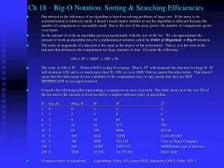
Ch 18 – Big-O Notation: Sorting & Searching Efficiencies • Our interest in the efficiency of an algorithm is based on solving problems of large size. If the array to be searched/sorted is relatively small, it doesn’t much matter whether or not the algorithm is efficient because the number of comparisons is reasonably small. But as the size of the array grows, the number of comparisons grows even faster. • So the amount of work an algorithm grows proportionally with the size of the list. We can approximate the amount of work an algorithm does by a mathematical notation called the Order of Magnitude or Big-Onotation. • The order of magnitude of a function is the same as the degree of the polynomial. That is, it is the term in the function that dominates the computation for large amounts of data. Consider the following: f(N) = N4 + 100N2 + 10N + 50 • The order of f(N) is N4 . Written O(N4) in Big-O notation. That is, N4 will dominate the function for large N. N4 will dominate f(N) and is so much more than 50, 10N, or even 100N2 that we ignore the other terms. That doesn’t mean that the other terms do not contribute to the computation time; it only means that they are NOT SIGNIFICANT in our approximation. • Consider the following table representing a comparison of rates of growth. The table shows how the size (N) of the list effects the amount of work needed to complete different types of algorithms. N log 2N Nlog2 N N2 N3 2N 1 0 0 1 1 2 2 1 2 4 8 4 4 2 8 16 64 16 8 3 24 64 512 256 16 4 64 256 4096 65,536 32 5 160 1024 32768 2,147,483,643 64 6 384 4096 362,144 5 yrs on Super Computer 128 7 896 16384 2.097,152 600000 times age of universe 256 8 2048 65,536 16,777,216 Don’t Ask! • Common orders of magnitude: Logarithmic O(log 2N), Linear O(N), Quadratic O(N2), Cubic O(N3)
SEARCHING Efficiencies using Big-O : Searching a phone book of 50,000 people. • Linear Search – A 50,000 element array would require 50,000 comparisons in a worst case scenario. The amount of work, comparisons, is in a direct correlation with the size of the list. • Binary Search – Is based on repeated divisions of 2. Consider the following: Divisions of 2 N=50,000 Fraction of List Mathematically Stated 1 25,000 1/2 2 12,500 1/4 The greatest number of comparisons will be K, 3 6,250 1/8 where K is the first value such that: 4 3,125 1/16 5 1,563 1/32 2K> N or 2K> 50,000 6 781 1/64 7 390 1/128 215 = 32,768 and 216 = 65,536 8 195 1/256 9 98 1/512 Written as a logarithm ( exp = logbaseanswer) 10 49 1/1024 11 24 1/2048 216 = 65,536 or 16 = log 265,536 12 12 1/4096 13 6 1/8192 Specifically for N = 50,000 14 3 1/16,384 log 250,000 = 15.6 15 2 1/32,768 16 1 1/65,536 • Therefore, the amount of work for a Binary Search is logarithmic in nature. The maximum number of comparisons of a 50,000 element array using the Binary Search would be 16! The only stipulation is that the list must be sorted first. • Summarizing our searching algorithms: • Sequential Search is an O(N) algorithm. • Binary Search is an O(log2 N) algorithm. Sometimes written as O(log N).
SIMPLE SORTING Efficiencies using Big-O • Selection/Exchange Sort : • Will always have N(N-1)/2 comparisons because it’s looping sequence of is always the same! for(int i=0; i<list.length-1 ; i++) for(int j=0; j<list.length ; j++) • Therefore, the Selection/Exchange Sorts order of magnitude is: • O(N2) • Bubble Sort - Consider the following more efficient version: int k = 1; //need at least 1 pass do{ sorted = true; for(int j = 0; j < list.length – k ; j++) if( list[j] > list[j+1] ){ swap(list, j); sorted = false; } k++; }while (!sorted); • Will have (2KN-K-K2 )/2 comparisons because it depends on the makeup of the array. • Since K is between 1 & N-1, we can say that K is on the same order as N. • 2KN will then dominate the function and is proportional to N2. • Therefore, the Bubble Sort order of magnitude is: • O(N2) • Which of these sorts is the most efficient on large amounts of data? • Because the Selection/Exchange Sort & Bubble Sort are both O(N2) algorithms, for large values of N there is NO SIGNIFICANT difference in the amount of work they do! The Bubble sort may require somewhat fewer comparisons, but the difference on average is not significant. • Most Simple Sorts are O(N2)
RECURSIVE SORTING Efficiencies using Big-O • QUICK SORT – The Quick Sort, like the Binary Search, uses the “divide & conquer” approach. The original list is divided into two lists. Each of these lists is again divided into two lists. This division continues until each list has exactly 1 element. Assuming that the splitting value is the median of the list, each sublist has approximately one-half as many elements as the previous list. It would therefore take up to log 2N levels of splits to complete. DataLevelOrder 1 0 O(N) 2 1 O(N) 4 2 O(N) 8 3 O(N) : : : N log2 N O(N) • At level 0, each number including the splitting value is compared to the splitting value. So N comparisons are made at level 0. • At level 1, there are two lists, one with k elements, and one with N-k elements. In the first list with k elements, k comparisons are made (each of the k elements to the new splitting value). In the second list of N-k elements, N-k comparisons are made. At level 1, a total of k + (N-k) or N comparisons are made. And so on for all levels. • Therefore, the total number of comparisons made to order a list of N elements using Quick Sort is the number of splitting levels log2N times the number of comparisons at each level N. • Consequently, the Quick Sort order of magnitude is O(Nlog2N).
Big-O Summary: Revisiting the rates of growth table from before: N log 2N Nlog2 N N2 N32N 1 0 1 1 1 2 2 1 2 4 8 4 4 2 8 16 64 16 8 3 24 64 512 256 16 4 64 256 4096 65,536 32 5 160 1024 32768 2,147,483,643 The order of magnitude, Big-O, of a function is the degree of the function. That is, it is the term that dominates the function for large size (N). This is an approximation that gives us a mathematical way to compare relative efficiencies for specific sorts & searches. Common Orders of Magnitude: O(N) Linear: Traversing a list sequentially one element at a time. O(log 2N) Logarithmic: Binary Search – Repeated divisions of 2. O(N2) Quadratic: Simple sorts. Traversing a 2-Dimensional array. O(N3) Cubic: Traversing a 3-Dimensional array. So what’s the most efficient algorithm in terms of Big-O notation: O(1) Constant Time: The size of the list doesn’t effect the time at all! Examples: Swapping data, accessing a component of an array through its index, inserting data into an array through its index. Hash tables arrange data so that they can be accessed directly through some ID number. In other words, their ID numbers have semantic meaning and are the indices of the array storing the data. Continued at a college near you!