Chap 7 Sorting
Chap 7 Sorting. The term list here is a collection of records. Each record has one or more fields. Each record has a key to distinguish one record with another.

Chap 7 Sorting
E N D
Presentation Transcript
Chap 7 Sorting
The term list here is a collection of records. Each record has one or more fields. Each record has a key to distinguish one record with another. For example, the phone directory is a list. Name, phone number, and even address can be the key, depending on the application or need. Motivation of Sorting
Two ways to store a collection of records Sequential Non-sequential Assume a sequential listf. To retrieve a record with key f[i].key from such a list, we can do search in the following order: f[n].key, f[n-1].key, …, f[1].key => sequential search Sorting
class Element { public: int getKey() const {return key;}; void setKey(int k) {key = k;}; private: int key; // other records … } Example of An Element of A Search List
int SeqSearch (Element *f, const int n, const int k) // Search a list f with key values // f[1].key, …, f[n].key. Return I such // that f[i].key == k. If there is no such record, return 0 { int i = n; f[0].setKey(k); while (f[i].getKey() != k) i--; return i; } Sequential Search
Sequential Search • The number of comparisons for a record key i is n – i +1. • The average number of comparisons for a successful search is • For the phone directory lookup, there should be a better way than this.
Search • A binary search only takes O(logn) time to search a sequential list with n records. • In fact, if we look up the name start with W in the phone directory, we start search toward the end of the directory rather than the middle. This search method is based on interpolation scheme. • An interpolation scheme relies on a ordered list.
void Verify1(Element* F1, Element* F2, const int n, const int m) // Compare two unordered lists F1 and F2 of size n and m, respectively { Boolean *marked = new Boolean[m]; for (int i = 1; i <= m; i++) marked[i] = FALSE; for (i = 1; i<= n; i++) { int j = SeqSearch(F2, m, F1[i].getKey()); if (j == 0) cout << F1[i].getKey() <<“not in F2 “ << endl; else { if (F1[i].other != F2[j].other) cout << “Discrepancy in “<<F[i].getKey()<<“:”<<F1[i].other << “and “ << F2[j].other << endl; marked[j] = TRUE; // marked the record in F2[j] as being seen } } for (i = 1; i <= m; i++) if (!marked[i]) cout << F2[i].getKey() <<“not in F1. “ << endl; delete [ ] marked; } Verifying Two Lists With Sequential Search O(mn)
void Verify2(Element* F1, Element* F2, const int n, const int m) // Same task as Verfy1. But sort F1 and F2 so that the keys are in // increasing order. Assume the keys in each list are identical { sort(F1, n); sort(F2, m); int i = 1; int j = 1; while ((i <= n) && (j <= m)) switch(compare(F1[i].getKey(), F2[j].getKey())) { case ‘<‘: cout<<F1[i].getKey() <<“not in F2”<< endl; i++; break; case ‘=‘: if (F1[i].other != F2[j].other) cout << “Discrepancy in “ << F1[i].getKey()<<“:” <<F1[i].other<<“ and “<<F2[j].other << endl; i++; j++; break; case ‘>’: cout <<F2[j].getKey()<<“ not in F1”<<endl; j++; } if (i <= n)PrintRest(F1, i, n, 1); //print records I through n of F1 else if (j <= m) PrintRest(F2, j, m, 2); // print records j through m of F2 } Fast Verification of Two Lists O(max{n log n, m log m})
Given a list of records (R1, R2, …, Rn). Each record has a key Ki. The sorting problem is then that of finding permutation, σ, such that Kσ(i)≤ K σ(i+1) , 1 ≤ i ≤ n – 1. The desired ordering is (Rσ(1), Rσ(2), Rσ(n)). Formal Description of Sorting
If a list has several key values that are identical, the permutation, σs, is not unique. Let σs be the permutation of the following properties: (1) Kσ(i)≤ K σ(i+1) , 1 ≤ i ≤ n – 1 (2) If i < j and Ki == Kj in the input list, then Ri precedes Rj in the sorted list. The above sorting method that generates σs is stable. Formal Description of Sorting (Cont.)
Internal Method: Methods to be used when the list to be sorted is small enough so that the entire sort list can be carried out in the main memory. Insertion sort, quick sort, merge sort, heap sort and radix sort. External Method: Methods to be used on larger lists. Categories of Sorting Method
void insert(const Element e, Element* list, int i) // Insert element e with key e.key into the ordered sequence list[0], …, list[i] such that the // resulting sequence is also ordered. Assume that e.key ≥ list[0].key. The array list must // have space allocated for at least i + 2 elements { while (e.getKey() < list[i].getKey()) { list[i+1] = list[i]; i--; } list[i+1] = e; } Insert Into A Sorted List O(i)
Insertion Sort void InsertSort(Element* list, constint n) // Sort list in nondecreasing order of key { list[0].setKey(MININT); for (int j = 2; j <= n; j++) insert(list[j], list, j-1); }
Insertion Sort Example 1 • Record Ri is left out of order (LOO) iff Ri< • Example 7.1: Assume n = 5 and the input key sequence is 5, 4, 3, 2, 1
Insertion Sort Example 2 • Example 7.2: Assume n = 5 and the input key sequence is 2, 3, 4, 5, 1 O(1) O(1) O(1) O(n)
If there are k LOO records in a list, the computing time for sorting the list via insertion sort is O((k+1)n) = O(kn). Therefore, if k << n, then insertion sort might be a good sorting choice. Insertion Sort Ananlysis
Binary insertion sort: the number of comparisons in an insertion sort can be reduced if we replace the sequential search by binary search. The number of records moves remains the same. List insertion sort: The elements of the list are represented as a linked list rather than an array. The number of record moves becomes zero because only the link fields require adjustment. However, we must retain the sequential search. Insertion Sort Variations
Quick sort is developed by C. A. R. Hoare. The quick sort scheme has the best average behavior among the sorting methods. Quick sort differs from insertion sort in that the pivot key Ki is placed at the correct spot with respect to the whole list. Kj≤ Ks(i) for j < s(i) and Kj ≥ s(i) for j > s(i). Therefore, the sublist to the left of S(i) and to the right of s(i) can be sorted independently. Quick Sort
void QuickSort(Element* list, constint left, constint right) // Sort records list[left], …, list[right] into nondecreasing order on field key. Key pivot = list[left].key is // arbitrarily chosen as the pivot key. Pointers I and j are used to partition the sublist so that at any time // list[m].key pivot, m < I, and list[m].key pivot, m > j. It is assumed that list[left].key ≤ list[right+1].key. { if (left < right) { int i = left, j = right + 1, pivot = list[left].getKey(); do { do i++; while (list[i].getKey() < pivot); do j--; while (list[j].getKey() > pivot); if (i<j) InterChange(list, i, j); } while (i < j); InterChange(list, left, j); QuickSort(list, left, j–1); QuickSort(list, j+1, right); } } Quick Sort
Quick Sort Example • Example 7.3: The input list has 10 records with keys (26, 5, 37, 1, 61, 11, 59, 15, 48, 19).
In QuickSort(), list[n+1] has been set to have a key at least as large as the remaining keys. Analysis of QuickSort The worst case O(n2) If each time a record is correctly positioned, the sublist of its left is of the same size of the sublist of its right. Assume T(n) is the time taken to sort a list of size n: T(n) ≤ cn + 2T(n/2), for some constant c ≤ ≤ cn + 2(cn/2 +2T(n/4)) ≤ 2cn + 4T(n/4) : : ≤ cn log2n + T(1) = O(n logn) Quick Sort (Cont.)
Lemma 7.1: Let Tavg(n) be the expected time for function QuickSort to sort a list with n records. Then there exists a constant k such that Tavg(n) ≤ kn logenfor n ≥ 2. Lemma 7.1
Unlike insertion sort (which only needs additional space for a record), quick sort needs stack space to implement the recursion. If the lists split evenly, the maximum recursion depth would be log n and the stack space is of O(log n). The worst case is when the lists split into a left sublist of size n – 1 and a right sublist of size 0 at each level of recursion. In this case, the recursion depth is n, the stack space of O(n). The worst case stack space can be reduced by a factor of 4 by realizing that right sublists of size less than 2 need not be stacked. Asymptotic reduction in stack space can be achieved by sorting smaller sublists first. In this case the additional stack space is at most O(log n). Analysis of Quick Sort
Quick sort using a median of three: Pick the median of the first, middle, and last keys in the current sublist as the pivot. Thus, pivot = median{Kl, K(l+r)/2, Kr}. Quick Sort Variations
So far both insertion sorting and quick sorting have worst-case complexity of O(n2). If we restrict the question to sorting algorithms in which the only operations permitted on keys are comparisons and interchanges, then O(n logn) is the best possible time. This is done by using a tree that describes the sorting process. Each vertex of the tree represents a key comparison, and the branches indicate the result. Such a tree is called decision tree. Decision Tree
Decision Tree for Insertion Sort K1 ≤ K2 No Yes K2 ≤ K3 K1 ≤ K3 No No Yes Yes stop K2 ≤ K2 stop K1 ≤ K3 No Yes No IV Yes I stop stop stop stop V VI II III
Theorem 7.1: Any decision tree that sorts n distinct elements has a height of at least log2(n!) + 1 Corollary: Any algorithm that sorts only by comparisons must have a worst-case computing time ofΩ(n log n) Decision Tree (Cont.)
void merge(Element* initList, Element* mergeList, const int l, const int m, const int n) { for (int i1 =l,iResult = l, i2 = m+1; i1<=m && i2<=n; iResult++){ if (initList[i1].getKey() <= initList[i2].getKey()) { mergeList[iResult] = initList[i1]; i1++; } else { mergeList[iResult] = initList[i2]; i2++; } } if (i1 > m) for (int t = i2; t <= n; t++) mergeList[iResult + t - i2] = initList[t]; else for (int t = i1; t <= m; t++) mergeList[iResult + t - i1] = initList[t]; } Simple Merge O(n - l + 1)
If an array is used, additional space for n – l +1 records is needed. If linked list is used instead, then additional space for n – l + 1 links is needed. Analysis of Simple Merge
O(1) Space Merge • A second merge algorithm only requires O(1) additional space. • Assume total of n records to be merged into a list, where n is a perfect square. And the numbers of records in the left sublist and the right sublist are multiple of
O(1) Space Merge Steps Step 1: Identify the records with largest keys. This is done by following right to left along the two lists to be merged. Step 2: Exchange the records of the second list that were identified in Step 1 with those just to the left of those identified from the first list so that the records with largest keys are contiguous. Step 3: Swap the block of largest with the leftmost block (unless it is already the leftmost block). Sort the rightmost block. Step 4: Reorder the blocks, excluding the block of largest records, into nondecreasing order of the last key in the blocks. Step 5: Perform as many merge substeps as needed to merge the blocks, other than the block with the largest keys. Step 6: Sort the block with the largest keys.
0 2 4 6 8 a c e g i j k l m n t w z|1 3 5 7 9 b d f h o p q r s u v x y 0 2 4 6 8 a c e g i j k l m n t w z 1 3 5 7 9 b d f h o p q r s u v x y 0 2 4 6 8 a|c e g i j k|uv x y w z|1 3 5 7 9 b|d f h o p q|r s l m n t u v x y wz|c e g i j k|0 2 4 6 8 a|1 3 5 7 9 b|d f h o p q|lm n r s t u v x y w z 0 2 4 6 8 a|1 3 5 7 9 b|c e g I j k|d f h o p q|l m n r s t 0 v x y w z u 2 4 6 8 a|1 3 5 7 9 b|c e g I j k|d f h o p q|l m n r s t 0 1 x y w z u 2 4 6 8 a|v 3 5 7 9 b|c e g I j k|d f h o p q|l m n r s t 0 1 2 y w z u x 4 6 8 a|v 3 5 7 9 b|c e g I j k|d f h o p q|l m n r s t O(1) Space Merge Example (First 8 Lines)
0 1 2 3 4 5 u x w 6 8 a|v y z 7 9 b|c e g i j k|d f h o p q|l m n r s t 0 1 2 3 4 5 6 7 8 u w a|v y z x 9 b|c e g i j k|d f h o p q|l m n r s t 0 1 2 3 4 5 6 7 8 9 a w|v y z x u b|c e g i j k|d f h o p q|l m n r s t 0 1 2 3 4 5 6 7 8 9 a w v y z x u b c e g i j k|d f h o p q|l m n r s t 0 1 2 3 4 5 6 7 8 9 a b c d e f g h i j k v z u|y x w o p q|l m n r s t 0 1 2 3 4 5 6 7 8 9 a b c d e f g h i j k v z u y x w o p q|l m n r s t 0 1 2 3 4 5 6 7 8 9 a b c d e f g h i j k l m n o p q y x w|v z u r s t 0 1 2 3 4 5 6 7 8 9 a b c d e f g h i j k l m n o p q r s t|v z u y x w O(1) Space Merge Example (Last 8 Lines)
Analysis of O(1) Space Merge • Step 1 and 2 and the swapping of Step 3 each take O( ) time and O(1) space. • The sort of Step 3 can be done in O(n) time and O(1) space using an insertion sort. • Step 4 can be done in O(n) time and O(1) space using a selection sort. (Selection sort sorts m records using O(m2) key comparisons and O(m) record moves. So it needs O(n) comparisons and the time to move blocks is O(n). • If insertion sort is used in Step 4, then the time becomes O(n1.5) since insertion sort needs O(m2) record moves ( records per block * n record moves).
Analysis of O(1) Space Merge (Cont.) • The total number of merge substeps is at most . The total time for Step 5 is O(n). • The sort of Step 6 can be done in O(n) by using either a selection sort or an insertion sort. • Therefore, the total time is O(n) and the additional space used is O(1).
Treat the input as n sorted lists, each of length 1. Lists are merged by pairs to obtain n/2 lists, each of size 2 (if n is odd, the one list is of length 1). The n/2 lists are then merged by pairs, and so on until we are left with only one list. Iterative Merge Sort
Merge Tree 26 5 77 1 61 11 59 15 48 19 5 26 1 77 11 61 15 59 19 48 1 5 26 77 11 15 59 61 19 48 1 5 11 15 26 59 61 77 19 48 1 5 11 15 19 26 48 59 61 77
void MergeSort(Element* list, const int n) // Sort list list into non-decreasing order of the keys list[1].key, …,list[n].key. { Element* tempList = new Element[n+1]; // l is the length of the sublist currently being merged. for (int l = 1; l < n; l *= 2) { MergePass(list, tempList, n, l); l *= 2; MergePass(tempList, list, n, l); //interchange role of list and tempList } delete[ ] tempList; } Iterative Merge Sort
void MergePass(Element* initList, Elemen* resultList, const int n, const int l) // One pass of merge sort. Adjacent pairs of sublists of length l are merged // from list initList to list resultList. n is the number of records in initList { for (int i = 1; i <= n – 2*l + 1; // Are enough elements remaining to form two sublists of length l? i += 2*l) merge(initList, resultList, i, i + l - 1, i + 2*l – 1); // merge remaining list of length < 2 * l if ((i + l – 1) < n) merge(initList, resultList, i, i+l–1, n); elsefor (int t = i; t <= n; t++) resultList[t] = initList[t]; } Merge Pass
Analysis of MergeSort • Total of passes are made over the data. Each pass of merge sort takes O(n) time. • The total of computing time is O(nlog n)
Recursive merge sort divides the list to be sorted into two roughly equal parts: the left sublist [left : (left+right)/2] the right sublist [(left+right)/2 +1 : right] These sublists are sorted recursively, and the sorted sublists are merged. To avoid copying, the use of a linked list (integer instead of real link) for sublist is desirable. Recursive Merge Sort
Sublist Partitioning For Recursive Merge Sort 26 5 77 1 61 11 59 15 48 19 5 26 11 59 19 48 5 26 77 11 15 59 19 48 1 61 1 5 26 61 77 11 15 19 48 59 1 5 11 15 19 26 48 59 61 77
class Element { private: int key; Field other; int link; public: Element() {link = 0;}; }; int rMergeSort(Element* list, const int left, const int right) // List list = (list[left], …, list[right]) is to be sorted on the field key. // link is a link field in each record that is initially 0 // list[0] is a record for intermediate results used only in ListMerge { if (left >= right) return left; int mid = (left + right)/2; return ListMerge(list, rMergeSort(list, left, mid), rMergeSort(list, mid+1, right)); } Program 7.11 (Recursive Merge Sort ) O(n log n)
int ListMerge(Element* list, const int start1, const int start2) { int iResult = 0; for (int i1 = start1, i2 = start2; i1 && i2;){ if (list[i1].key <= list[i2].key) { list[iResult].link = i1; iResult = i1; i1 = list[i1].link; } else { list[iResult].link = i2; iResult = i2; i2 = list[i2].link; } } // move remainder if (i1 == 0) list[iResult].link = i2; else list[iResult] = i1; return list[0].link; } Program 7.12 (Merging Linked Lists)
Natural merge sort takes advantage of the prevailing order within the list before performing merge sort. It runs an initial pass over the data to determine the sublists of records that are in order. Then it uses the sublists for the merge sort. Natural Merge Sort
Natural Merge Sort Example 26 5 77 1 61 11 59 15 48 19 5 26 77 1 11 59 61 15 19 48 1 5 11 26 59 61 77 15 19 48 1 5 11 15 19 26 48 59 61 77
Merge sort needs additional storage space proportional to the number of records in the file being sorted, even though its computing time is O(n log n) O(1) merge only needs O(1) space but the sorting algorithm is much slower. We will see that heap sort only requires a fixed amount of additional storage and achieves worst-case and average computing time O(n log n). Heap sort uses the max-heap structure. Heap Sort
For heap sort, first of all, the n records are inserted into an empty heap. Next, the records are extracted from the heap one at a time. With the use of a special function adjust(), we can create a heap of n records faster. Heap Sort (Cont.)
void adjust (Element* tree, const int root, const int n) // Adjust the binary tree with root root to satisfy the heap property. The left and right subtrees of root // already satisfy the heap property. No node has index greater than n. { Element e = tree[root]; int k = e.getKey(); for (int j = 2*root; j <= n; j *= 2) { if (j < n) if (tree[j].getKey() < tree[j+1].getKey()) j++; // compare max child with k. If k is max, then done. if (k >= tree[j].getKey()) break; tree[j/2] = tree[j]; // move jth record up the tree } tree[j/2] = e; } Program 7.13 (Adjusting A Max Heap)