Presentation Transcript

1. Introduction to Network Mathematics (2)- Probability and Queueing

   YuedongXu 10/08/2012
2. Purpose All networking systems are stochastic Analyzing the performance of a protocol (e.g. TCP), a strategy (peer selection), a system (e.g. Data center), etc.
3. Outline Probability Basics Stochastic Process Baby Queueing Theory Statistics Application to P2P Summary
4. A and B B A Probability Basics Review Probability: a way to measure the likelyhood that a possible outcome will occur. Between 0 and 1 Events A and B AUB: union AB: intersection A UB
5. Probability Basics Review (‘cont) P(AUB): prob. that either A or B happen P(AUB) = P(A) + P(B) – P(AB) P(A|B): prob. that A happens, given Bs P(A|B) = P(AB)/P(B) P(AB): prob. that both A and B happen P(AB) = P(A|B)*P(B) = P(B|A)*P(A)
6. Probability Basics If A and B are mutually exclusive P(AB) = 0 P(AUB) = P(A) + P(B) P(A|B) = 0 If A and B are independent P(AB) = P(A)*P(B) P(AUB) = P(A) + P(B) - P(A)*P(B) P(A|B) = P(A)
7. Probability Basics Review (‘cont) Theorem of total probability: Events {Bi, i=1,2,…,k} are mutually exclusive.
8. Probability Basics Review (‘cont) Bayesian's Theorem Suppose that B1, B2, … Bk form a partition of S: Then
9. “n factorial” Probability Basics Review (‘cont) A permutation is an ordered arrangement of objects. The number of different permutations of n distinct objects is n!. n! = n · (n – 1)· (n – 2)· (n – 3)· …· 3· 2· 1 Example: How many different surveys are required to cover all possible question arrangements if there are 7 questions in a survey? 7! = 7 · 6 · 5 · 4 · 3 · 2 · 1 = 5040 surveys
10. Probability Basics Review (‘cont) The number of permutations of n elements taken r at a time is # in the group # taken from the group Example: You are required to read 5 books from a list of 8. In how many different orders can you do so?
11. Probability Basics Review (‘cont) A combination is a selection of r objects from a group of n things when order does not matter. The number of combinations of r objects selected from a group of n objects is # in the collection # taken from the collection Example: You are required to read 5 books from a list of 8. In how many different ways can you do so if the order doesn’t matter?
12. Probability Basics Review (‘cont) Discrete random variable (r.v.) Binomial distribution, Poisson distribution, and so on
13. Probability Basics Review (‘cont) Continuous random variable Uniform distribution, Normal distribution, Gamma distribution, and so on
14. Probability Basics We enter the more advanced phase! Never get confused by the concepts!
15. Probability Basics Key Concepts Probability mass function (pmf) Used for discreter.v. Suppose that X: S → A is a discrete r.v. defined on a sample space S. Then the probability mass function fX: A → [0, 1] for X is defined as
16. Probability Basics Key Concepts Probability density function (pdf) i) Used for continuousr.v.; ii) A function that describes the relative likelihood for this r.v. to take on a given value. A random variable X has density f, where f is a non-negative Lebesgue-integrable function, if:
17. Probability Basics Key Concepts Cumulative distribution function (cdf) For a discrete r.v. X For a continuous r.v. X
18. Probability Basics Key Concepts Probability generating function (pgf) i) Used for discrete r.v. ii) A power series representation of pmf For a discrete r.v. X where p is the probability mass function of X.
19. Probability Basics Key Concepts Moment generating function (mgf): a way to represent probability distribution What is “moment” of the r.v. X? kth moment E[Xk]
20. Probability Basics Key Concepts The moment-generating function of r.v. X is wherever this expectation exists. Why is mgf extremely important? unified way to represent the high-order properties of a r.v. such as expectation, variance, etc.
21. Probability Basics Key Concepts In the college study, we know how to compute Mean and variance of a r.v. The joint distribution of two or more r.v.s But, they are studied case by case! Any unified approach?
22. Probability Basics Key Concepts Major properties of mgf Calculating moments Mean: E(X) = MX(1)(0) Variance: E(X) = MX(2)(0) –(MX(1)(0))2
23. Probability Basics Key Concepts Major properties of mgf ii) Calculating distribution of sum of r.v.s Given independent r.v.sX1 and X2, and the sum Y = X2+X2, what is the distribution of Y? If we know the mgf MX1(n) and MX2(n), then MY(n) = MX1(n) *MX2(n)
24. 1-p = probability of failure p = probability of success r := # successes out of n trials Probability Basics Commonly Used Distributions Binomial distribution: if you have only two possible outcomes (call them 1/0 or yes/no or success/failure) in n independent trials, then the probability of exactly r “successes”=
25. Probability Basics Commonly Used Distributions mgf of Binomial distribution:
26. Probability Basics Commonly Used Distributions mgf of Binomial distribution:
27. Probability Basics Commonly Used Distributions Exponential distribution: a continuous r.v. whose pgf has Example: 1/lambda is the mean duration of waiting for the next bus if the bus arrival time is exponentially distributed.
28. Probability Basics Commonly Used Distributions mgf of exponential distribution:
29. Probability Basics Commonly Used Distributions mgf of exponential distribution:
30. Probability Basics Commonly Used Distributions Continuous r.v.
31. Probability Basics Commonly Used Distributions Discrete r.v.
32. Probability Basics Advanced Distributions in Networking Power law distribution Intuitive meaning: The prob. that you have 1 Billion USD is extremely small (continuous example) Lin Dan (x=1 badminton player) gets much more media exposure than an unknown one with x=10 (discrete example)
33. Probability Basics Advanced Distributions in Networking Power law distribution Intuitive meaning: The prob. that you have 1 Billion USD is extremely small (continuous example) Lin Dan (x=1 badminton player) gets much more media exposure than an unknown one with x=10 (discrete example)
34. Probability Basics Examples of power-law Word frequency Paper citations Web hits P2P file poplarity Wealth of the richest people. Frequencies of surnames Populations of cities.
35. Probability Basics Laplace and Z-transform Laplace transform is essentially the m.g.f. of non-negative r.v. Z-Transform (ZT) is the m.g.f. of a discrete r.v. The purpose is to compute the distribution of r.v.s in a easier way
36. Probability Basics Laplace transform The moments can again be determined by differentiation: LT of a sum of independent r.v.s is the product of LTs No need to compute the convolutions one by one!
37. Probability Basics Take home messages Moment generating function is vital in computing probability distribution Laplace transform (and Z transform) has many applications
38. Probability Basics Sub-summary Review basic knowledge of probability Highlight important concepts Review some commonly used distributions Introduce Laplace and Z transforms
39. Outline Probability Basics Stochastic Process Baby Queueing Theory Statistics Application to P2P Summary
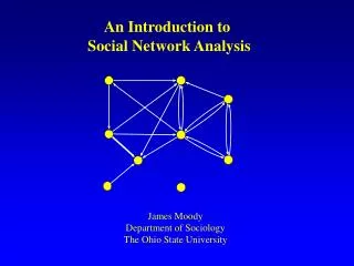
40. Stochastic Process Concepts Random variance: a standalone variable Stochastic process: a stochastic process X(t) is a family of random variables indexed by a time parameter t a random variable for each fixed t a sample path X(t) t time
41. Stochastic Process To be more accurate, A stochastic process N= {N(t), t T} is a collection of r.v., i.e., for each t in the index set T, N(t) is a random variable t: time N(t): state at time t If T is a countable set, N is a discrete-time stochastic process If T is continuous, N is a continuous-time stochastic process
42. Stochastic Process Counting process A stochastic process {N(t) ,t  0} is said to be a counting process if N(t) is the total number of events that occurred up to time t. Hence, some properties of a counting process is N(t)  0 N(t) is integer valued If s < t, N(t)  N(s) For s < t, N(t) – N(s) equals number of events occurring in the interval (s, t]
43. Stochastic Process Poisson process Def. A: the counting process {N(t), t0} is said to be Poisson process having rate l, l>0 if N(0) = 0; The process has independent-increments Number of events in any interval of length t is Poisson dist. with mean lt, that is for all s, t 0.
44. Stochastic Process Markov process Q: What is Markov process? Is it a new process? A: No, it refers to any stochastic process that satisfies the Markov property!
45. Stochastic Process Markov process P[X(tn+1)  Xn+1| X(tn)= xn, X(tn-1) = xn-1,…X(t1)=x1] = P[X(tn+1)  Xn+1| X(tn)=xn] Probabilistic future of the process depends only on the current state, not on the history We are mostly concerned with discrete-space Markov process, commonly referred to as Markov chains Discrete-time Markov chains Continuous-time Markov chains
46. Stochastic Process Discrete Time Markov Chain P[Xn+1= j | Xn= kn, Xn-1 = kn-1,…X0= k0] = P[Xn+1 = j | Xn= kn] discrete time, discrete space a finite-state DTMC if its state space is finite a homogeneous DTMC if P[Xn+1= j | Xn= i ] does not depend on n for all i, j, i.e., Pij = P[Xn+1= j | Xn= i ], where Pij is one step transition prob.
47. 0.95 A B C D 0.95 0 0.05 0 0.2 0.5 A A B 0.2 0.5 0 0.3 B 0.2 0.3 0.05 0.8 0 0.2 0 0.8 D C C 1 0 0 1 0 D Stochastic Process Discrete Time Markov Chain P = [ Pij] is the transition matrix transition probability Representation as a directed graph
48. Stochastic Process Continuous Time Markov Chain Continuous time, discrete state P[X(t)= j | X(s)=i, X(sn-1)= in-1,…X(s0) = i0] = P[X(t)= j | X(s)=i] A continuous M.C. is homogeneous if P[X(t+u)= j | X(s+u)=i] = P[X(t)= j | X(s)=i] = Pij[t-s], where t > s Chapman-Kolmogorovequation
49. A B C D -0.1 0 0.1 0 0.2 A A B 0.2 -0.5 0 0.3 B 0.2 0.3 0.1 0.8 0 0.2 -1 0.8 D C C 1.2 0 0 1.2 -1.2 D Stochastic Process Continuous Time Markov Chain P = [ Pij] is called intensity matrix transition rate Representation as a directed graph
50. E B A A B D D C C Stochastic Process Continuous Time Markov Chain Irreducible Markov chain: a Markov Chain is irreducibleif the corresponding graph is strongly connected. irreducible reducible
51. E A B D C Stochastic Process Continuous Time Markov Chain Ergodic Markov chain: a Markov Chain is ergodic if i) strongly connected graph; ii) not periodic. Some periodic behaviors in the transitions from A->B->C->D Not Ergodic
52. Stochastic Process Continuous Time Markov Chain Ergodic Markov chain: a Markov Chain is ergodic if i) strongly connected graph; ii) not periodic. Ergodic Markov Chains are important since they guarantee the corresponding Markovianprocess converges to a unique distribution, in which all states have strictly positive probability. A B D C Ergodic
53. Stochastic Process Steady State - DTMC: Let π = (π1, π2, . . . , πm) is the m-dimensional row vector of steady-state (unconditional) probabilities for the state space S = {1,…,m}. (e.g. m=3) π1 + π2 + π2 = 1, π1 0, π2 0, π3 0 transition probability Solve linear system: π = πP, πj= 1, πj 0, j = 1,…,m
54. Stochastic Process Steady State – CTMC The computation is based on Flow balance equation. Will be highlighted in the following slides: Baby queueing theory
55. Stochastic Process Sub-summary Stochastic process is a collection of r.v.s. indexed by time Markov process refers to the stochastic processes that the future only depends on the current state.
56. Outline Probability Basics Stochastic Process Baby Queueing Theory Statistics Application to P2P Summary
57. Baby Queueing Theory Queueing theory is the most important tool (not one of) to evaluate the performance of computing systems (Kleinrock) “We study the phenomena of standing, waiting, and serving, and we call this study Queueing Theory." "Any system in which arrivals place demands upon a finite capacity resource may be termed a queueing system.”
58. Baby Queueing Theory You want to know quick and insightful answers to Delay Delay variation (jitter) Packet loss Efficient sharing of bandwidth Performance of variaous traffic type (audio/video, file transfer, interactive) Call rejection rate Performance of packet/flow scheduling And so on ……
59. Baby Queueing Theory Our slides will cover Basic terms of queueing theory Basic queueing models Basic analytical approachs and results Basic knowledge of queueing networks Application to P2P networks
60. Baby Queueing Theory Basic terms Arrival and service are stochastic processes Customers Server Queue Queuing System
61. Baby Queueing Theory Basic terms Arrival Process M: Markovian D: Deterministic Er: Erlang G: General Service Process M: Markovian D: Deterministic Er: Erlang G: General A/B/m/K/N Number of servers m=1,2,… Number of customers N= 1,2,… (for closed networks otherwise it is omitted) Storage Capacity K= 1,2,… (if ∞ then it is omitted)
62. Baby Queueing Theory Basic terms We are interested in steady state behavior Even though it is possible to pursue transient results, it is a significantly more difficult task. E[S] average system time (average time spent in the system) E[W] average waiting time (average time spent waiting in queue(s)) E[X] average queue length E[U] average utilization (fraction of time that the resources are being used) E[R] average throughput (rate that customers leave the system) E[L] average customer loss (rate that customers are lost or probability that a customer is lost)
63. λj-1 λ0 λ1 λj λ2 λj-2 j-1 j 0 1 2 μj+1 μ3 μj-1 μj μ1 μ2 Baby Queueing Theory M/M/1 – Steady state Meaning: Poisson Arrivals, exponentially distributed service times, one server and infinite capacity buffer. (here, λj=λ andμj=μ) At steady state, we obtain (due to flow balance)
64. Solution exists if Baby Queueing Theory M/M/1 – Steady state In general Making the sum equal to 1 Letting λj=λ andμj=μ, we have for λ/μ = ρ <1
65. Baby Queueing Theory M/M/1 - Performance Server Utilization Throughput Expected Queue Length
66. Baby Queueing Theory M/M/1 - Performance Average System Time Average waiting time in queue
67. Baby Queueing Theory M/M/1 - Example μ=0.5 rho=λ/μ Ε[S] Ε[W] Ε[Χ]
68. a(t) d(t) Area γ(t) N(t) Time t Baby Queueing Theory Little’s Law – obtaining delay a(t): the process that counts the number of arrivals up to t. d(t): the process that counts # of departures up to t. N(t)=a(t)- d(t) Average arrival rate (up to t)λt= a(t)/t Average time each customer spends in the system Tt= γ(t)/a(t) Average number in the system Nt= γ(t)/t
69. a(t) Area γ(t) d(t) N(t) Time t Baby Queueing Theory Little’s Law – obtaining delay Taking the limit as t goes to infinity Expected number of customers in the system Expected time in system Arrival rate IN the system
70. λ λ λ λ λ λ m m+1 0 1 2 mμ 3μ mμ mμ μ 2μ 1 … m Baby Queueing Theory M/M/m – Steady state Meaning: Poisson Arrivals, exponentially distributed service times, midentical servers and infinite buffer.
71. Baby Queueing Theory M/M/m – Steady state The analysis can be done using flow balance equations (in the same way as M/M/1) How can we compare M/M/1 to M/M/m? What are the insights we can get?
72. μ2 λ μ1 μ2 λ Β μ3 Α μ3 λ C Baby Queueing Theory M/M/m vs M/M/1 Suppose that customers arrive according to a Poisson process with rate λ=1. You are given three options, Install a single server with processing capacity μ1= 1.5 Install two identical servers with processing capacity μ2= 0.75and μ3= 0.75 Split the incoming traffic to two queues each with probability 0.5 and have μ2= 0.75and μ3= 0.75serve each queue.
73. Baby Queueing Theory M/M/m vs M/M/1 Throughput It is easy to see that all three systems have the same throughput E[RA]= E[RB]= E[RC]=λ Server Utilization Therefore, each server is 2/3 utilized Therefore, all servers are similarly loaded.
74. Baby Queueing Theory M/M/m vs M/M/1 Probability of being idle For each server
75. Baby Queueing Theory M/M/m vs M/M/1 Queue length and delay For each queue!
76. λ λ λ λ λ K-1 K 0 1 2 μ μ μ μ μ Baby Queueing Theory M/M/1/K Meaning: Poisson Arrivals, exponentially distributed service times, one server and finite capacity buffer K. Using the birth-death resultλj=λ andμj=μ, we obtain Therefore for λ/μ = ρ
77. Baby Queueing Theory M/M/1/K - Performance Server Utilization Throughput Blocking Probability Probability that an arriving customer finds the queue full (at state K)
78. Baby Queueing Theory M/M/1/K - Performance Expected Queue Length Net arrival rate (no losses) System time
79. Baby Queueing Theory More difficult queueing models M/G/1 G/M/1 G/G/1 In other words, if the inter-arrival time, or the service time follow a more general distribution, the performance analysis is more challenging. Then, we may using various approximation techniques to obtain the asymptotic behaviors
80. Baby Queueing Theory Queueing Networks Single queue is usually not enough to model complicated job scheduling, or packet delivery Queueing Network: model in which jobs departing from one queue arrive at another queue (or possibly the same queue)
81. Baby Queueing Theory Open queueing network Jobs arrive from external sources, circulate, and eventually depart What is the delay of traversing multiple queues?
82. Baby Queueing Theory Closed queueing network Machine repairman problem
83. Baby Queueing Theory Example 1 – Tandem network kM/M/1 queues in series Each individual queue can be analyzed independently of other queues Arrival rate=l. If mi is the service rate for ith server:
84. Baby Queueing Theory Example 1 – Tandem network Joint probability of queue lengths: product form network!
85. Baby Queueing Theory Insights Queueing networks are in general very difficult to analyze, even intractable! If each queue can be analyzed independently, we might be lucky to analyze the queueing networks in product-form ! Next objective: what kinds of queues own this product-form property?
86. Baby Queueing Theory Jackson networks Jackson (1963) showed that any arbitrary open network of m-server queues with exponentially distributed service times has a product form In general, the internal flow in such networks is not Poisson, in particular when there are feedbacks in the network.
87. Baby Queueing Theory BCMP networks Gordon and Newell (1967) showed that any arbitrary closed networks of m-server queues with exponentially distributed service times also have a product form solution Baskett, Chandy, Muntz, and Palacios (1975) showed that product form solutions exist for an even broader class of networks (no matter it is an open or closed one)
88. Baby Queueing Theory BCMP networks k severs R 1 classes of customers Customers may change class Allowing class changes means that a customer can have different mean service rates for different visits to the same node.
89. Baby Queueing Theory BCMP networks Sever may be only of four types: First-come-first-served (FCFS) Processor sharing (PS) Infinite servers (IS or delay centers) and Last-come-first-served-preemptive-resume (LCFS-PR) Still quite limited!
90. Baby Queueing Theory Relationships of queueing networks Product Form Networks Denning&Buzen BCMP Jackson
91. Baby Queueing Theory Sub-summary Little’s law: mean delay = mean # of jobs/service rate Flow balance approach to solve CTMC Classic Queueing models and their performance Only product-form queueing networks are not difficult to be analyzed
92. Outline Probability Basics Stochastic Process Baby Queueing Theory Statistics Application to P2P Summary
93. Statistics
94. Outline Probability Basics Stochastic Process Baby Queueing Theory Statistics Application to P2P Summary
95. Summary Basic knowledge of probability Moment generating function, Laplace trans. Basic stochastic processes Solving steady state of Markov chain Baby queueing theory M/M/1, M/M/m, M/M/1/K, Jackson, BCMP Statistics To be added
96. Thanks!
97. Probability Basics Advanced Distributions in Networking Zipf distribution: Named after George Zipf Describing frequency of occurrence of words Very useful in characterizing File popularity Keyword occurrence Importance of nodes and so on …… George Kingsley Zipf 1902-1950
98. Probability Basics Advanced Distributions in Networking Zipf distribution: the high the rank, the lower the frequency of occurrence. N: the number of elements; k : their rank; s : the exponential parameter
99. Probability Basics Advanced Distributions in Networking Zipf distribution: example