Continuous Word Recognition
Database. text. speech. text. text. text. Scoring. Continuous Word Recognition. Continuous Word Recognition. Problems with isolated word recognition: we don´t know the limits of the words. Increases variability coarticulation of “words” Speech velocity.

Continuous Word Recognition
E N D
Presentation Transcript
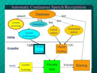
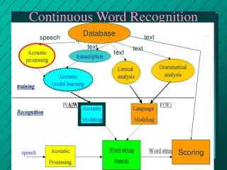
Database text speech text text text Scoring Continuous Word Recognition
Continuous Word Recognition • Problems with isolated word recognition: • we don´t know the limits of the words. • Increases variability • coarticulation of “words” • Speech velocity
Issues in the choice of subword units sets • Context Independent: Phonemes • Few, easy to train. • A HMM is to poor to take into account the phone context variability. • SPHINX: model_architecture/Telefonica.ci.mdef • Context Dependent:Triphone: • Phonemes in a specific context at left and right. • Very Larger number of units to train. • Very Large quantity of training data needed. • SPHINX: model_architecture/Telefonica.untied.mdef
Clustering Acoustic-Phonetic Units • Many Phones have similar effects on the neighboring phones, hence, many triphones have very similar Markov states. • A senone is a cluster of similar Markov states. • Advantages: • More training data. • Less memory used.
Senonic Decision Tree (SDT) • SDT Classify Markov States of Triphones represented in the training corpus by asking Linguistic Questions composed of Conjuntions, Disjunctions and/or negations of a set of predetermined
Decision Tree for Classifying the second state of k-triphone Is left phone (LP) a sonorant or nasal? yes Is left phone /s,z,sh,sh/? Is right phone (RP) a back-R? Is RF voiced? Senone 5 Senone 1 Senone 6 Is LP back L or ( LC neither a nasal or RF A LAX-vowel)? Senone 4 Senone 3 Senone 2
When applied to the word welcome Is left phone (LP) a sonorant or nasal? yes Is left phone /s,z,sh,sh/? Is right phone (RP) a back-R? Is RF voiced? Senone 5 Senone 1 Senone 6 Is LP back L or ( LC neither a nasal or RF A LAX-vowel)? Senone 4 Senone 3 Senone 2
The tree can automatically constructed by searching, for each node, the question that the maximum entropy decrease • Sphinx: • Construction: $base_dir/ c_scripts/03.bulidtrees. • Results: $base_dir/trees/Telefonica.unpruned/A-0.dtree • When the tree grows, it needs to be pruned • Sphinx: • $base_dir/ c_scripts/ 04.bulidtrees. • Results:aA • $base_dir/trees/Telefonica.500/A-0.dtree • $base_dir/Telefonica_arquitecture/Telefonica.500.mdef
Words • Words can be modeled using composite HMMs • A null transition is used to go from one subword unit to the following /sil/ /uw/ /sil/ /t/
Database text speech text text text Scoring Continuous Speech Training
For each utterance to train, the subword units are concatenated to form words model. • Sphinx: Dictionary • $base_dir/training_input/dict.txt • We can estimate parameters using the forward-backward reestimation formulas already described.
The ability to automatically align each individual HMM to the corresponding unsegmente speech observation sequence is one of the most powerfull features in the forward-backward algorithm.
Database text speech text text text Scoring
Language Models for Large Vocabulary Speech Recognitin • Goal: • Provide an estimate of the probability of a “word” sequence (w1 w2 w3 ...wQ) for the given recognition task. • This can be solved as follows:
Since, it is impossible to reliable estimate the conditional probabilities, • hence in practice it is used an N-gram language model: • En practice, realiable estimators are obtained for N=1 (unigram) N=2 (bigram) or possible N=3 (trigram). j
Examples: • Unigram: • P(Maria loves Pedro)=P(Maria)P(loves)P(Pedro) • Bigram: • P(Maria|<sil>)P(loves|Maria)P(Pedro|loves)P(</sil>|Pedro)
CMU-Cambridge Language Modeling Tools • $base_dir/c_scripts/languageModelling
Database text speech text text text Scoring
C(Wi-2 Wi-1 Wi ) P(Wi| Wi-2,Wi-1)= C(Wi-2 Wi-1) where C(Wi-2 Wi-1 )=Total Number Sequence Wi-2 Wi-1 was observed C(Wi-2 Wi-1 Wi ) =Total Number Sequence Wi-2 Wi-1 Wi was observed
Database text speech text text text Scoring
0.1 0.3 0.2 0.2 0.3 0.5 0.7 0.8 0.3 0.5 0.9 0.4 0.5 0.1 0.6 1.0 1.0 1.0 0.3 0.5 0.6 0.7 0.3 0.2 Unigram P(Wi)
Bigram P(Wi| Wi-1) merge Word 1 Acoustic model Null state Null state expand Word 2 Acoustic model Null state Null state Null state Word n Acoustic model Null state
0.1 0.3 0.2 0.2 0.3 0.5 0.7 0.8 0.3 0.5 0.9 0.4 0.5 0.1 0.6 1.0 1.0 1.0 0.3 0.5 0.6 0.7 0.3 0.2 Viterbi Algorithm
1. Inicialisation: 2. Calculate every state of every model using: t.probj+log(aij) 3. Update every internal state of every model: max(t.probj+log(aij)) 4. Update state N of every model: 5. Find mode with higher logProbability 0.3 0.2 0.2 0.1 0.7 0.3 0.2 0.5 0.1 0.5 6. Update limits table 1.0 1.0 0.7 0.5 0.3 0.7 2.5 0 0.0 0 Inf 0 -Inf 0 -Inf 0 7. Copy token in state 1 of each model. 5.3 0 4.5 0 4.5 0 1.2 0 3.2 0 2.1 0 5.3 0 4.5 0 2.2 0 2.7 0 5.2 0 4.5 0 0.0 0 Inf 0 -Inf 0 -Inf 0 2.7 0 4.5 0 2.3 0 3.5 0 4.3 0 2 0 4.5 0 7.3 0 4.5 0 1.3 0 Each state as a token t t.probj t.startj • frame at which the token at • state j enter the model w.model 1 0 w.start
0.1 0.3 0.2 0.2 0.3 0.5 0.7 0.8 0.3 0.5 0.9 0.4 0.5 0.1 0.6 1.0 1.0 1.0 0.3 0.5 0.6 0.7 0.3 0.2 For N words
Recovering the uttered words. • Array w, is the same length as the number of observations. • This array gives information of the limits of the words. • At the end of the utterance, value w.model[M] stores the last HMM recognised sequence, and the predecesor models are obtain by “tracking back” trough the array.
Finite State Syntax (FSS) • With token passing the FSS are straightforward implemented. Monterrey Monterrey to Frankfort Frankfort from Houston Houston
Large Vocabulary Continuous Speech Recognition • Problems with isolated word recognition: • Do not easily account for variations in word pronunciation accross different dialects, etc. • Solution: • Use subword speech units. • Problems with large vocabulary continuous Speech Recognition: • we don´t know the limits of the subword units. • Increases variability • coarticulation of subword units • Speech velocity
La probabilidad MAP (Maximum A Posteriory) de la cadena de palabras W dadas la observaciones: • Utilizando la regla de Bayes:
ya que P(O) es independiente de W • Modelo Acústico: • Sub-palabras. • PhoneLike Units(PLU):50 • Syllable-like Units (SLU): 10,000 • Dyad: 2000 • Acusticas (Clustering): 256-512 • Lenguaje Model: • Restricciones • Sintácticas: • “parser” o • n-gram (n=2,3,4) • Par de palabras (word pair) • semánticas del Lenguaje.
Smoothing • Since many trigrams are rarerly found, even in large amount of text. Smoothing is used as follows:
0.1 0.3 0.2 0.2 0.3 0.5 0.7 0.8 0.3 0.5 0.9 0.4 0.5 0.1 0.6 1.0 1.0 1.0 0.3 0.5 0.6 0.7 0.3 0.2 Recognition
1. Inicialisation: 2. Calculate every state of every model using: t.probj+log(aij) 3. Update every internal state of every model: max(t.probj+log(aij)) 4. Update state N of every model: 5. Find mode with higher logProbability 0.3 0.2 0.2 0.1 0.7 0.3 0.2 0.5 0.1 0.5 6. Update limits table 1.0 1.0 0.7 0.5 0.3 0.7 2.5 0 0.0 0 Inf 0 -Inf 0 -Inf 0 7. Copy token in state 1 of each model. 5.3 0 4.5 0 4.5 0 1.2 0 3.2 0 2.1 0 5.3 0 4.5 0 2.2 0 2.7 0 5.2 0 4.5 0 0.0 0 Inf 0 -Inf 0 -Inf 0 2.7 0 4.5 0 2.3 0 3.5 0 4.3 0 2 0 4.5 0 7.3 0 4.5 0 1.3 0 Each state as a token t t.probj t.startj • frame at which the token at • state j enter the model w.model 1 0 w.start
0.1 0.3 0.2 0.2 0.3 0.5 0.7 0.8 0.3 0.5 0.9 0.4 0.5 0.1 0.6 1.0 1.0 1.0 0.3 0.5 0.6 0.7 0.3 0.2 For N subunits
Recovering the uttered words. • Array w, is the same length as the number of observations. • This array gives information of the limits of the words. • At the end of the utterance, value w.model[M] stores the last HMM recognised sequence, and the predecesor models are obtain by “tracking back” trough the array.
Finite State Syntax (FSS) • With token passing the FSS are straightforward implemented. Monterrey Monterrey to Frankfort Frankfort from Houston Houston
Initial Estimates • Reestimation equations give parameter values which converge to a local maximum. • Experience shown that • aijparameters converge to the global parameter without problem. • state distribution function (bi,o(t) ) or parameters (mean and variance) need good initial estimates. • Segmental k-means Segmentation into States
Segmental k-means Segmentation into states Chosen randomly or any available model. Using Viterby Algorithm and back tracking. Number of vectors k bj(k)= Number of vectors in j. m =Mean of the vector in the state j j s =Mean of the vector in the state j j
State Duration HMM Modelling • For most physical signals, the exponential distribution is inappropriate. • In order to improve modeling, we have to incorporate state duration information in a HMM. • Incorporate state duration information into the mechanics of HMMs. • Heuristic method.
Heuristic for incorporating state duration into HMM • At training: • Segmental k-means algorithm is used. • Calculate the state duration probability pj(d). • At recognition: • Viterbi algorithm to obtain • The logProbability and • the best segmentation via backtracking. • The duration of each state is measure from the state segmentation. • A post processor increases the logProbability as follows:
0.00477 0.0 0.0 0.024 0.01008 0.00954 0.0 0.0 0.28 0.0204 0.00311 0.0 0.8 0.16 0.00256 0.00005 0.0 0.0 0.0 0.0 Implementation Advise • If the number of models, in the decoding process, is very large, then try to save memory. Observe that for a given time t, it only need a limited quantity of information: s t
s 0.00477 0.00932 0.0 0.0 0.0 0.0 0.037 0.024 0.01008 0.02008 0.0154 0.00954 0.0 0.0 0.0 0.0 0.28 0.61 0.0204 0.074 0.00561 0.00311 0.0 0.0 0.8 0.8 0.16 0.32 0.00256 0.0046 0.00025 0.00005 0.0 0.0 0.0 0.0 0.0 0.0 0.0 0.0 s
s s 0.0133 0.01972 0.0035 0.00932 0.0 0.0 0.0 0.0 0.0 0.0 0.0 0.0 0.037 0.037 0.037 0.037 0.02008 0.02008 0.02008 0.02008 0.0154 0.0154 0.0154 0.0154 0.0 0.0 0.0 0.0 0.0 0.0 0.0 0.0 0.61 0.61 0.61 0.61 0.074 0.074 0.074 0.074 0.00561 0.00561 0.00561 0.00561 0.0 0.0 0.0 0.0 0.8 0.8 0.8 0.8 0.32 0.32 0.32 0.32 0.00025 0.00025 0.00025 0.0046 0.0046 0.0046 0.0046 0.00025 0.0 0.0 0.0 0.0 0.0 0.0 0.0 0.0 0.0 0.0 0.0 0.0 0.0 0.0 0.0 0.0 s s