Download
1 / 56
570 likes | 742 Vues
Simulation of the Operation of the ITER Coils using a Domain Decomposition Method. D. Bessette , L. Bottura, A. Devred , J. Persichetti , F. Gauthier CHATS-AS XI CERN, October 12 th -14 th 2011. Outline. A domain decomposition ? Practical implementation

E N D
Simulation of the Operation of the ITER Coils using a Domain Decomposition Method D. Bessette, L. Bottura, A. Devred, J. Persichetti, F. Gauthier CHATS-AS XI CERN, October 12th-14th 2011
Outline • A domain decomposition ? • Practical implementation • The ITER CS coil – a test problem • Other results and further work • ITER PF coils • ITER TF coils • Summary and perspective
Outline • A domain decomposition ? • Practical implementation • The ITER CS coil – a test problem • Other results and further work • ITER PF coils • ITER TF coils • Summary and perspective
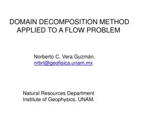
http://en.wikipedia.org/wiki/Domain_decomposition_methods Domain Decomposition Sigh… • […] domain decomposition methods solve a boundary value problem by splitting it into smaller boundary value problems on subdomains and iterating to coordinate the solution between adjacent subdomains […] which makes domain decomposition methods suitable for parallel computing
Which decomposition ? • Different physics domains are strongly coupled on comparable time scales • Geometric proximity (space domains) and difference of characteristic times (time scale domain) are more suitable for a domain decomposition • The building bricks are attacking different sets of combined physics on physically coherent objects
The physics domains HEATER FLOWER POWER THEA M’C
Outline • A domain decomposition ? • Practical implementation • The ITER CS coil – a test problem • Other results and further work • ITER PF coils • ITER TF coils • Summary and perspective
Child 1 Child 2 Child n Implementation • Link independent simulation processes (children) through a communication protocol for data exchange • A single master program (father) manages generation of each process, synchronization, and communication Father Child 1 Child 2 … Child n Father and Child processes is a concept borrowed from unix
THEA POWER manager POWER THEA THEA FLOWER manager POWER THEA manager DATA interpolation manager HEATER manager FLOWER FLOWER HEATER HEATER HEATER HEATER FLOWER Overall structure SUPERMAGNET
Sample coupling – 1/2 Coupling node HEATER line HEATER point HEATER node HEATER element
Sample coupling – 2/2 Coupling node HEATER line T <> q’’ HEATER point FLOWER junction T <> q’’ T <> q’’ FLOWER volume T <> q’’ THEA thermal T <> q’’ THEA hydraulic
Linear interpolation of point results in time to exchange data at intermediate time stations Bi-linear interpolation of line results in space and time to exchange data between different meshes and at intermediate time stations Data interpolation Un U mesh n U* tn x U Un+1 required time t* mesh n+1 tn+1 x* x required position t
Outline • A domain decomposition ? • Practical implementation • The ITER CS coil – a test problem • Other results and further work • ITER PF coils • ITER TF coils • Summary and perspective
The ITER CS • Winding pack (WP) consisting of 240 pancakes • cold mass: 700 t • cooling path (one pancake): 150m • supply/return feeders from CTB to WP: 53m • 4 main cryolines CTB to ACB: 40m, 95m • Circulator (pump): 2 kg/s • Heat exchanger: 4.2K
CS conductor CS CICC originally designed for operating at 40 kA, 13T, 4.5K with a T margin higher (or equal) to 0.7K Copper content sufficient to limit the hot spot temperature below 150K in case of fast discharge of 7.5 s time constant triggered by a quench
15 MA Scenario v1.10 Conductor current End of Rebias (t=1790s) 40.0 kA at SOD SOD (t=0) EOB (t=500s) 45.4 kA at 516s
15 MA Scenario v1.10 Magnetic field and strain 40 kA, 12.96 T B map and Strain map are established from the conductor current and the coil layout. Peak values of I, dI/dt, B, dB/dt are generally not coincident in time, space I, B operating window Local Strain IxB dependence is included (derived from TFJA4 test at 1000 cycles) (%) = -0.74 – 1.3 e-4 BI with I (kA), B(T) Potential benefit of the hoop strain not included Contour plot of Bpeak a SOD
15 MA Scenario v1.10 AC loss Consider (Jc, Qhyst) of strands selected for the CS conductor (e.g. Hitachi) Two approaches for coupling losses: models by E. Zapretilina https://user.iter.org/?uid=2FVJB7 • Single time constant model (conservative), nTau = 100ms, Qcoupl 60%, Qhyst 40% - 8.1 MJ total losses • Varying time constant model (most realistic), saturation completed at cycle nr 10,000 Qcoupl 40%, Qhyst 60% - 6.4 MJ total losses
Self field effect Definition of Beff 1. compute: 2. solve iteratively:
FLOWER model of CS J3 V8 J1 J4 J2 V9 V7 V6 V5 CS1U J12 V15 V21 J18 V2 J421…J500 V4 J11 V14 CS2U V20 J17 J341…J420 J6 J20 J10 V13 CS3U V19 J16 J261…J340 J9 V12 CS3L V18 J15 J181…J260 V1 V3 J8 V11 CS2L V17 J14 J101…J180 J5 J19 J7 V10 CS1L V16 J13 J21…J100
The typical “mechanical” mesh requires a relatively fine level of detail (mm) to capture large gradients in stress/strain This level of detail (about 10000 elements per x-section !) is not practical for the thermal analysis Thermal meshing issues
The “thermal” mesh required is much coarser for the type of system-scale analysis targeted This is the maximum level of detail recommended (about 500 elements per x-section) Typical maximal mesh Parabolic, 8-nodes, iso-parametric elements
Example of CS Hexa-pancake geometry - edges and lines “edges” 23712 Nodes 6588 Elements 8016 Edges line
Model of CS module 2 fluid channels 1 conductor component 200 nodes per channel 240 THEA processes Approximately 1 MDOFs 24 hrs execution time for 1800 s 8 sections 106656 nodes 30504 quad elements 35520 line edges 6 HEATER processes 21 volumes 500 junctions 1 FLOWER process
CS simulation heat balance • Approximate calculation of the total energy in- and outflow (pump work, enthalpy difference, neglect energy stored in heat capacity) • estimated 2.5 % “discrepancy” on the overall balance – quite good
HX temperatures HX inlet HX outlet • Heat transfer coefficient taken as constant (500 W/m2K) • Inner surface 2 m2 • Outer surface 6 m2
Pressure bumps during operation HX inlet HX outlet • Pressure flexes correspond to changes in heating power • Relatively large pressure excursions and heating induced backflow
3-D maps at 3600 s 4.58 K 4.38 K
3-D maps at 3610 s 4.66 K 4.89 K 5.47 K
3-D maps at 3700 s 5.17 K 4.80 K 5.66 K
CS results – first cycle CS2U Pancake 173 Restarted 4 times during the 1800 s of simulation
CS results – following cycles CS2U Pancake 173 Detail of the first 10 s of simulation
Outline • A domain decomposition ? • Practical implementation • The ITER CS – a test problem • Other results and further work • PF coils • TF coils • Summary and perspective
FLOWER model of PF coils 85 volumes 580 junctions PF windings CCS CCT CCB
HEATER models of PF Example of PF1 32768 nodes 25864 elements 17760 edges 160 lines 2-in hand pancakes
PF Manifolds temperatures Inlet manifolds Outlet manifolds Cryoplant manifolds
PF coil temperatures PF1 Pancake 1 1st in hand PF3 Pancake 1 1st in hand PF6 Pancake 1 1st in hand
Outline • A domain decomposition ? • Practical implementation • The ITER CS – a test problem • Other results and further work • PF coils • TF coils • Summary and perspective
TF mesh example No difference among pancakes (yet) Conceptually simple However, complexity is significant 139854 nodes 42856 parabolic elements 26992 edges
TF mesh details Jacket Conductor insulation Plate Ground insulation
Summary • Displace on the user’s side the parameterization of the system analyzed • PRO: generic code(s), e.g. number of strands in the cable, topology of the coil, cooling mode, field and AC loss dependence on lengthand time, without the need to “recompile” • CON: logistics of a large size system becomes heavy, easy to get lost • Big is out, small and modular is in • PRO: The good Father directs many Children, and finds its reward in the details the work of every single one • CON: The control-freak Manager spends most of his time dealing with the details of every Slave process (also called micro-management, watch-out for a “Banker’s Bonus”) • Lots can be done, do we really need it ? • Ah, by the way, why “SuperMagnet” ?
1987 – C. Marinucci at SIN computes B, AC loss, temperatures in a plasma burn scenario using a code sequence named “Phase1, Phase2, Phase3,…”: the first power user of the codes is born • 1989-1995 – monolithic analysis codes (SARUMAN, GANDALF) and first attempts to couple domains • 1995 – V. Arp at Cryodata distributes CryoSoft codes under the package name of Supermagnetpak (akin to Hepak, Gaspak, Metalpak, Expak, Cppak). I admit I did not like the name • 1997 – C. Luongo and B. Parsons (Bechtel) perform design and analysis of a superconducting system using codes operated in sequence (M’C, OPTICON, ZERODEE) and advocate the need for an integrated system of codes for SC magnet design and analysis • 2001 – THEA • 2008 – HEATER • Challenge launched in 2008 by the ITER magnet project leader (“you will not manage to simulate the ITER system”) vs. a bottle of good French Wine. SuperMagnet is born