Multi-Dimensional Arrays
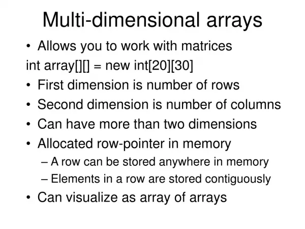
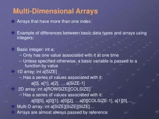
Multi-Dimensional Arrays. Matrices. Arrays seen so far are single dimensional A linear list of items One subscript for accessing individual elements Multidimensional arrays are useful organizations in many applications values of temperatures at different locations in different times

Multi-Dimensional Arrays
E N D
Presentation Transcript
Matrices • Arrays seen so far are single dimensional • A linear list of items • One subscript for accessing individual elements • Multidimensional arrays are useful organizations in many applications • values of temperatures at different locations in different times • number of runs in different sessions on different days in a test match • trajectory of a planet in space - time • Matrices • simplest and useful multidimensional arrays • Two dimensions
Two-Dimensional Data Structures • Fortran allows variables that can assume two dimensional array values • Typical values are: 23 14 95.6 78.9 23.2.true. .true. 12 67 894.7 0.7 15.2.false. .false. 9 5 566.0 98.2 76.5.true. .true. 5.2 23.0 14.6 • An integer 3 by 3 matrix: 3 rows and 3 columns of integer values • 4 by 3 real matrix • 3 by 2 logical matrix
Matrix Declaration • Matrix entries can be of different types • No. of rows and columns can be arbitrary • Fortran Declaration defines these two attributes for a matrix variable • Real,Dimension(3,6):: Sum • Logical,Dimension(23:100,-2:5):: flag • integer,Dimension(15:19,5):: runs • Accessing an element • Sum(2,5), flag(56,0), runs(18,3) • Two subscripts are needed
Matrix Representation • Memory is Single-Dimensional • Linear representation of matrix elements • Row major order: One row after another • Column major order: one column after another (assumed representation) • Example: 15 56 67 76 20 54 77 11 3 45 86 22 15 20 3 56 54 45 67 77 86 76 11 22
Initialization/Assignment • Using array constructor (column major order) A = (\ 2,3,4,3,4,5,4,5,6 \) • Explicit nested do loops do I = 1, 5 do J = 1,8 A(I,J) = I + J end do end do • Whole row/column assignment do I =1,5 A(I,:) = I end do • Initialization can be done at the time of declaration
Assignment • Whole, part or individual array elements can be assigned A = ... A(:,i) = ... A(i,j) = … • The rhs should be appropriate type • Lifting of scalar to suitable types may be required • with READ statements read *, ((A(i,j),j = 1, 3), I = 1, 4)
Using matrix variables • Matrix variables can be accessed, individually, in sections or as a whole • Used in expressions on the right hand side of any assignment • Intrinsic functions on base types lifted to matrix types • Eg. Abs, Sin, Cos, Tan, Log, Sqrt can be applied to a matrix variable • Sin(A) is a similar matrix in which each entry is Sin of the corresponding entries in A
Other intrinsic functions • LBOUND(A,d) – lower bound of index in the dimension d • LBOUND(A) - list of lower bounds • UBOUND - upper bound, similar • SIZE(A,d) - number of entries in dimension d • size(A) - total no. of elements • SHAPE(A) - returns the `shape' of A • Extent in a dimension is the no. of entries in that dimension • Shape is an one dimensional array of extents(one entry per dimension)
Transformational Intrinsic Functions • Dot_Product(A,B) - dot product of one dimensional arrays of A and B • MATMUL(A,B) - Matrix multiplication on conformable matrices A and B • RESHAPE(A,B) - B is a one-dimensional shape array • Entries in A are converted into an array of shape B • Column major order used • Example: Suppose A = 2 5 6 7 and B = [6,2] 1 3 2 8 7 5 8 9 • Reshape(A,B) = 2 7 3 6 8 8 1 5 5 2 7 9 • Usually used for initializing a matrix from a linear list of elements
Masked Assignment • A more generalized selection is possible using WHERE construct • Suppose, you want to multiply all entries > 0 by 2, and all other entries set to 0 then where (A > 0) A = 2 * A elsewhere A = 0 end where • Note: Reference to an array has many connotations – context dependent
Accessing Matrix variables • When a matrix is accessed, the index values should be valid • illegal values lead to run-time error - Array index exceeding bounds • Compiler optionally inserts code for the check
Generalized Arrays • Multi-dimensional arrays are possible • All array operations, like declaration, initialization and use are similar • Rank of an array is the number of dimensions • One-dimensional array is of rank 1, matrix of rank 2 etc. • Arrays of up to rank 7 are allowed in Fortran
Memory Allocation • Arrays are allocated memory by the compiler • The allocation is static - done at compile time • More and larger arrays, larger the memory requirement • Array use and their size requirements should be done with care • indiscriminate use would result in wastage of memory • Use arrays only when all the data in the arrays are required at the same time in memory
Allocatable Arrays • Allocatable arrays is a solution to memory wastage problem • When the size of an input data set is unknown, better to use the following: real, dimension(), allocatable :: A integer, dimension(:), allocatable :: B • This is a declaration of an Array A and B of rank 1 and 2 respectively • Only ranks specified, the extent decided dynamically • When A ( and B) initialized, the extents are decided and allocated • This enables avoiding static allocation of conservative estimate of required space
Allocate Construct • Allocatable arrays are allocated memory using explicit instruction: allocate(A(n), i) • This indicates the extent of A is the value of n • This is an external routine that may succeed or fail • Succeeds when the memory allocation is successful • The external procedure sends a value 0 via the parameter i • Typically the size is input by the user which is used in the allocation • Allocated memory can be deallocated using deallocate(A,i) • This succeeds provided the value returned via i is 0
Illustration Linear Systems of Equations • Most commonly occurring problem, the original motivation for matrices • solve a system of n equations in n variables a11x1 + a12x2 + ... + a1nxn = b1 a12x2 + a22x2 + ... + a2nxn = b2 ... an1x1 + an2x2 + … + annxn = bn • aij,, bj are all real numbers
Gaussian Elimination • choose any equation and any variable with non zero coefficient ( called pivot) in the equation • eliminate this variable from all other equations by adding a multiple of chosen equation • repeat with remaining equations • solve one equation in one variable • back substitute value of variable to find others • two steps, elimination and back substitution
Program real, dimension(:,:), allocatable :: a integer :: n, i, j real, dimension(:), allocatable :: x read *, n ! Number of variables allocate(x(n), stat=i) if ( i /= 0) then print *, "allocation of x failed" stop endif allocate(a(n,n+1), stat=i) if ( i /= 0) then print *, "allocation of array a failed" stop endif do i = 1,n print *, "enter coefficients of equation", i read *, a(i, 1:n+1) end do
do i = 1,n a(i, i:n+1) = a(i,i:n+1)/a(i,i)! make coefficient of x_i 1.0 do j = i+1,n a(j,i:n+1) = a(j,i:n+1) - a(i,i:n+1)*a(j,i) end do ! eliminate x_i end do do i = n, 1, -1 x(i) = a(i,n+1) - sum(a(i,i+1:n)*x(i+1:n)) end do ! sum of a null array is 0.0 print *, "solution is" print *, x(1:n) deallocate(a, x, stat=i) if ( i /= 0) then print *, "deallocation failed" stop endif
Elimination • a(1:n+1,1:n+1) contains the coefficients, x(1:n) the computed values of variables • assumes a(i,i) /= 0.0 at every step • true for many special types of matrices • problem if abs(a(i,i)) is too small • elimination needs to be done only once for different right hand sides • only back substitution needs to be done • reduces operations from n3 to n2
Pivoting • swap rows and columns to make a(i,i) large • partial pivoting - swap row i with row containing maxval(abs(a(i:n,i))) • what if it is 0.0? • complete pivoting- swap row and column to make a(i,i) = maxval(abs(a(i:n,i:n))) • what if it is still 0.0? • this changes order of the variables • gives more accurate results but more time