Introduction to Scientific Visualization
Introduction to Scientific Visualization. CS 4390/5390 Data Visualization Shirley Moore, Instructor October 13, 2014. SciVis aka Spatial Data Visualization.

Introduction to Scientific Visualization
E N D
Presentation Transcript
Introduction to Scientific Visualization CS 4390/5390 Data Visualization Shirley Moore, Instructor October 13, 2014
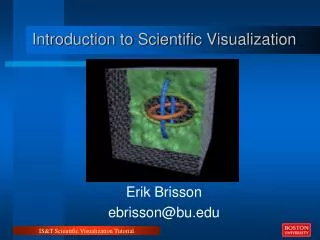
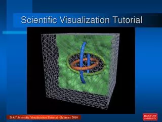
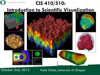
SciVis aka Spatial Data Visualization • SciVis emerged as a discipline in the 1980s in response to the large amount of data produced by numerical simulations of physical phenomena (e.g., fluid flow, heat convection, material deformation). • Primary concern is visualization of 3D phenomena with emphasis on realistic renderings of volumes, surfaces, illuminations source, etc. • Depiction of datasets that have a natural spatial embedding • Relies heavily on computer graphics • Reference: Data Visualization: Principles and Practice, by AlexandruTelea, 2nd edition, CRC Press, 2014.
SciVis Pipeline Image credit: AlexandruTelea, Data Visualization: Principles and Practice, 2nd edition
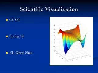
Simple Example: Visualization of a Scalar Function of Two Variables
Sample 1 Code in C++ and GLUT • sample1.cpp • What happens if we use fewer sample points? • Viewpoint of virtual camera
Rendering Equation • Describes relationship between incoming light, outgoing light, and material properties at a given point • Approximate lighting effects to varying degrees of realism • Global illumination methods • radiosity methods • ray-tracing methods • Local illumination methods • Phong lighting model
Phong-Blinn Lighting Model • Bui-TuongPhong, “Illumination for Computer-Generated Images”, 1973 • Jim Blinn, “Models of Light Reflections for Computer Synthesized Pictures”, 1977
Phong-Blinn Lighting Model (2) Image from Wikipedia Phong lighting equation: I(p, v, L) = cambIl(cdiffmax(-L. n, 0) + cspecmax(r. v, 0)α)
Phong Lighting Model in OpenGL • With flat shading: sample3.cpp • With Gouraud shading: sample4.cpp
Transparency • Draw domain grid: sample5.cpp • Draw elevation plot with transparency factor: sample6.cpp
Texture Mapping • Map 2D texture image onto 3D elevation plot • Sample7.cpp
ParaView • http://www.paraview.org/ • Open source tool for scientific data visualization • Collaborative project between Kitware, Los Alamos National Lab, Sandia National Lab, and Army Research Lab • Can run in parallel to process large datasets • Built on top of the Visualization Toolkit (VTK), which is a portable open source C++ library for computer graphics and visualization • http://www.vtk.org/ • Flat and Gouraud shading examples in ParaView: • Gaussian (flat).pvsm • Gaussian (Gouraud).pvsm
Preparation for Next Class • Finish Lab 3 • Study for quiz