Read Me!
This article discusses the steps involved in quantifying and analyzing alcohol-related phenotypes, focusing on the correction of errors due to brain shrinkage, multiple raters, and extraneous variables. Linear regression is proposed as a method to control for these variables.

Read Me!
E N D
Presentation Transcript
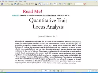
Read Me! Grisel JE. Quantitative trait locus analysis.Alcohol Res Health. 2000;24(3):169-74.
Bioinformatics/Neuroinformatics Unit—Specific steps • Quantify phenotype—olfactory bulb volume • Remove error variance • Due to differential shrinkage of brains • Due to multiple raters • Due to extraneous variables--demographic characteristics (eg. Sex, age, body weight, brain weight) and other individual differences.
Now that the phenotype has been quantified, we need to clean up these data! First of all, who shrank the brains?
OK--so we have to correct for shrinkage in case it is variable among brains, which it is.
We can correct for the shrinkage ifwe know the density of brain (1.05 mg/mm3) because we know how much the brain weighed before processing. We can figure out its original volume, then correct for shrinkage of the olfactory bulbs using this formula:
Bioinformatics/Neuroinformatics Unit—Specific steps • Quantify phenotype—olfactory bulb volume • Remove error variance • Due to differential shrinkage of brains • Due to multiple raters • Due to extraneous variables--demographic characteristics (eg. Sex, age, body weight, brain weight) and other individual differences.
We are getting rid of error due to multiple raters by: using multiple measurers for each mouse--and insisting that these raters agree. 2) using the median value of all measurers of a given mouse.
Bioinformatics/Neuroinformatics Unit—Specific steps • Quantify phenotype—olfactory bulb volume • Remove error variance • Due to differential shrinkage of brains • Due to multiple raters • Due to extraneous variables--demographic characteristics (eg. Sex, age, body weight, brain weight) and other individual differences.
So, you have quantified the phenotype, Let’s get on with it!
What a mess! Why did you guys use mice of different sexes, ages, body weights, and brain weights? Didn’t your professors ever teach you anything about controls????
HI! I’m Francis Galton, Chuck Darwin’s cousin, and I can help you out of this mess! You need one of my inventions, linear regression, to help you with your lack of control there, Gregor.
By the way, I called it regression, because everybody seemed to regress toward the mean through successive generations!
Obviously, you can’t control for sex, body weight, brain weight, and age at this point! But thanks to me, you can control for these variables by a statistical method--linear regression. Using linear regression allows one to eliminate the variance (differences) in scores associated with these various extraneous variables.
Fortunately, we can assume that variance--statistics talk for the differences among individuals-- is additive.
What is key in using regression to control for various extraneous variables is the additive model of variance. s2total=s2sex+s2bodyweight + s2brainweight+ s2age +s2error + s2olfactorybulb genes
Thus, the total variance can be partitioned into the variance associated with each of these extraneous variables such as sex, body weight, brain weight, and age. Then we can successively remove the variance associated with each of these variables and hopefully just have residual variance that only pertains to gene effects on olfactory bulbs.
Let us first consider the case of simple linear regression before we tackle the problem of multiple regression.
In regression we predict the y variable from the x.
In regression we predict the y variable from the x.
Residual (error) _ ^ Y OB Volume Y Variance predicted by X Body Weight (grams)
The variance left over after the variance from the other variable(s) has been removed is the residual variance. This residual variance is precious to us because it has the variance specific gene effects on olfactory bulbs.
So the SSE SSyy is our treasure, yet another’s trash.
By using multiple regression, We can remove the variance associated with extraneous variables and so statistically control for these variables.
What is key in using regression to control for various extraneous variables is the additive model of variance. s2total=s2sex+s2bodyweight + s2brainweight+ s2age +s2error + s2olfactorybulb genes
Not yer data! Variables Controlled by Regression
Bioinformatics/Neuroinformatics Unit—Specific steps • Quantify phenotype—olfactory bulb volume • Remove error variance • Due to differential shrinkage of brains • Due to multiple raters • Due to extraneous variables--demographic characteristics (eg. Sex, age, body weight, brain weight) and other individual differences.
Bioinformatics/Neuroinformatics Unit—Specific steps • Quantify phenotype—olfactory bulb volume • Remove error variance • Due to differential shrinkage of brains • Due to multiple raters • Due to extraneous variables--demographic characteristics (eg. Sex, age, body weight, brain weight)and other individual differences.
Regression must be done on individuals. After having controlled for various variables by regression, we will average the olfactory bulb values from the various individuals within a given recombinant inbred strain.
Recall, however, that we can think of Each Measurement = Error + True Score s2error + s2olfactorybulb genes
If our measures largely error, then relationships with variance in the phenotype with variance in the genome will be watered-down because error tends to work randomly and add noise to our data. Randomness cannot be systematically related to anything.
How to make mistakes with statistics • Type II (beta) errors—AKA false negatives • Small effect size • Small n • Greater variance in scores • Greater the error variance, the more Type II errors • Type I (alpha) errors—false positives • Stringency of the alpha error rate • Significant Individual point p = 1.5 x 10⁻⁵ for genome-wide a = .05 • Suggested individual point p = 3 x 10⁻⁴ for genome wide a = .63
QTL is good for detecting the approximate locus of multiple genes affecting a phenotype across all the chromosomes, except Y. This is a graph that displays the likelihood ratio statistic as a function of locus on the various chromosomes, which are numbered at top.
Thus, lots of error variance will give us false negatives (Type II errors) when we do QTL analyses!
LRS is LOW X all B D B D B B D D B X B B B D Phenotypic Measurement (Residual) D B X D B D D D B D D B D B D B Marker Type
LRS is High X B X all X D D D D D D D D D D D D D Phenotypic Measurement (Residual) B B B B B B B B B B B B D B Marker Type
LRS is LOW X all B D B D B B D D B X B B B D Phenotypic Measurement (Residual) D B X D B D D D B D D B D B D B Marker Type
We may not replicate Williams et al. for a couple of reasons.
Williams et al. used weight, which is a more objective measure than ours and had fewer observers. Thus, they probably had less error associated with their measures and fewer false negatives (Type II errors).
We excluded all of the anterior olfactory nucleus, whereas Williams et al. (2001) cut through it in an irregular fashion.
In this lecture you have learned about 1) simple and multiple regression and how they can be used to control for extraneous variables, 2) how error is being controlled in your experiment 3) Reasons why you may not have perfectly replicated Williams et al. (2001).
On behalf of your mentors, do enjoy the remains of the day.