CS263 : Lecture 7 – Advanced SQL

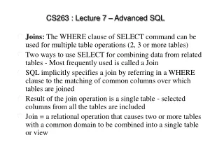
1. CS263 : Lecture 7 – Advanced SQL Joins: The WHERE clause of SELECT command can be used for multiple table operations (2, 3 or more tables) Two ways to use SELECT for combining data from related tables - Most frequently used is called a Join SQL implicitly specifies a join by referring in a WHERE clause to the matching of common columns over which tables are joined Result of the join operation is a single table - selected columns from all the tables are included Join = a relational operation that causes two or more tables with a common domain to be combined into a single table or view

2. Joins Each row returned contains data from rows in the different input tables where values for the common columns match An important rule of thumb: there should be one condition within the WHERE clause for each pair of tables being joined. If two tables are combined, one condition would be necessary, but if three tables (A, B, C) are to be combined, then two conditions would be necessary because there are two pairs of tables (A-B and B-C) There are several types of joins, the most commonly used are the following 4:

3. Equi-join Equi-join – a join in which the joining condition is based on equality between values in the common columns; common columns appear redundantly in the result table e.g. if we want to know the names of customers who have placed orders, that information is kept in 2 tables CUSTOMER_T and ORDER_T. If we want to find the names of customers who have placed orders: SELECT CUSTOMER_T.CUSTOMER_ID, ORDER_T.CUSTOMER_ID, CUSTOMER_NAME, ORDER_ID FROM CUSTOMER_T, ORDER_T WHERE CUSTOMER_T.CUSTOMER_ID = ORDER_T.CUSTOMER_ID;

4. Natural join An equi-join where one of duplicate columns is eliminated in result table (most commonly used form of join operation) From the previous example, one CUSTOMER_ID would be left out Notice that CUSTOMER_ID must still be qualified as it exists in both CUSTOMER_T and ORDER_T e.g. for each customer who placed an order, what is the customer’s name and order number? SELECT CUSTOMER_T.CUSTOMER_ID, CUSTOMER_NAME, ORDER_ID FROM CUSTOMER_T, ORDER_T WHERE CUSTOMER_T.CUSTOMER_ID = ORDER_T.CUSTOMER_ID

5. Outer join • Often find that row in one table does not have a matching row in the other table • e.g., several CUSTOMER_ID numbers may not appear in the ORDER_T table (maybe they have not ordered for a long time) • As a result, the equi-join and natural join do not include all of the customers in CUSTOMER_T • Using an outer join rows that do not have matching values in common columns are also included in the result table. Null values appear in columns where there is not a match between the tables • (as opposed to inner join, in which rows must have matching values in order to appear in the result table)

6. e.g. List the customer name, ID number, and order number for all customers. Include customer information even for customers that do have an order: SELECT CUSTOMER_T.CUSTOMER_ID, CUSTOMER_NAME, ORDER_ID FROM CUSTOMER_T, LEFT OUTER JOIN ORDER_T WHERE CUSTOMER_T.CUSTOMER_ID = ORDER_T.CUSTOMER_ID Syntax LEFT OUTER JOIN selected as CUSTOMER_T named first, and is table from which we want all rows (regardless of whether there is matching order in the ORDER_T table) If we reversed order tables were listed, same results could be obtained using a RIGHT OUTER JOIN Also possible to request a FULL OUTER JOIN - all rows matched and returned, including any that do not have a match in the other table

7. Union join Includes all columns from each table in the join, and an instance for each row of each table, i.e. the result of a union join is a table that includes all of the data from each table that is joined So a union join of the CUSTOMER_T table (15 customers and 6 attributes) and the ORDER_T table (10 orders and 3 attributes) will return a results table of 25 rows and 9 columns Assuming that each original table contained no nulls, each customer row in the results table will contain 3 attributes with assigned null values and each order row will contain 6 attributes with assigned null values Do not confuse this command with the UNION command for joining select STATEMENTS (discussed later)

8. Sample multiple join with 4 tables This query on the next page produces a result table that includes all the information needed to create an invoice for order no. 1006. We want the customer information, the order information, the order line information and the product information (4 tables) Since the join involves 4 tables, there will be 3 column join conditions Each pair of tables requires an equality-check condition in the WHERE clause, matching primary keys against foreign keys Joining useful when data from several relations are to be retrieved, and the relationships are not necessarily nested

9. 4 table join • SELECT CUSTOMER_T.CUSTOMER_ID, CUSTOMER_NAME, CUSTOMER_ADDRESS, CITY, SATE, POSTAL_CODE, ORDER_T.ORDER_ID, ORDER_DATE, QUANTITY, PRODUCT_NAME, UNIT_PRICE, (QUANTITY * UNIT_PRICE) • FROM CUSTOMER_T, ORDER_T, ORDER_LINE_T, PRODUCT_T • WHERE CUSTOMER_T.CUSTOMER_ID = ORDER_LINE.CUSTOMER_ID AND ORDER_T.ORDER_ID = ORDER_LINE_T.ORDER_ID AND ORDER_LINE_T.PROUCT_ID = PRODUCT_PRODUCT_ID AND ORDER_T.ORDER_ID = 1006;

10. From CUSTOMER_T table From PRODUCT_T table From ORDER_T table Results from a four-table join

11. Subqueries (nested subqueries) • Placing an inner query (SELECT, FROM, WHERE) within a WHERE or HAVING clause of another (outer) query • The inner query provides values for the search condition of the outer query • There can be multiple levels of nesting • Useful alternative to joining when there is nesting of relationships • The following queries both answer the question ‘what is the name and address of the customer who placed order number 1008?’ • The second version uses the subquery technique

12. Subqueries SELECT CUSTOMER_NAME, CUSTOMER_ADDRESS, CITY, STATE, POSTAL_CODE FROM CUSTOMER_T, ORDER_T WHERE CUSTOMER_T.CUSTOMER_ID = ORDER_T.CUSTOMER_ID AND ORDER_ID = 1008; ------------------------------------------------------------------------

13. Subqueries SELECT CUSTOMER_NAME, CUSTOMER_ADDRESS, CITY, STATE, POSTAL_CODE FROM CUSTOMER_T WHERE CUSTOMER_T.CUSTOMER_ID = (SELECT ORDER_T.CUSTOMER_ID FROM ORDER_T WHERE ORDER_ID = 1008);

14. Subqueries The subquery approach may be used for this query because we only need to display data from the table in the outer query The value for ORDER_ID does not appear in the query result - it is used as a selection criterion in the outer query To include data from the subquery in the result, we should use a join technique (since data from a subquery cannot be included in the final results)

15. Subqueries • Another example - ‘which customers have placed orders’ • The IN operator will test to see if the CUSTOMER_ID value of a row is included in the list returned from the subquery • Subquery is embedded in parentheses. In this case it returns a list that will be used in the WHERE clause of the outer query. DISTINCT is used because we do not care how many orders a customer has placed as long as they have placed an order • SELECT CUSTOMER_NAME FROM CUSTOMER_T • WHERE CUSTOMER_ID IN (SELECT DISTINCT CUSTOMER_ID FROM ORDER_T);

16. Subqueries Following example shows use of NOT and demonstrates using a join in an inner query ‘Which customers have not placed any orders for computer desks?’ SELECT CUSTOMER_NAME FROM CUSTOMER_T WHERE CUSTOMER_ID NOT IN (SELECT CUSTOMER_ID FROM ORDER_T, ORDER_LINE_T, PRODUCT_T WHERE ORDER_T.ORDER_ID = ORDER_LINE_T.ORDER_ID AND ORDER_LINE_T.PRODUCT_ID = PRODUCT_T.PRODUCT_ID AND PRODUCT_NAME = ‘Computer Desk’);

17. Subqueries So here the inner query returned a list of all customers who had ordered computer desks The outer query listed the names of those customers who were not in the list returned by the inner query EXISTS and NOT EXISTS can be used in the same location where IN would be (just prior to the beginning of the subquery) EXISTS will take a value of ‘true’ if the subquery returns an intermediate results table which contains one or more values, and ‘false’ if no rows are returned (the opposite for NOT EXISTS)

18. Subqueries e.g. ‘what are the order numbers for all orders that have included furniture finished in natural ash?’ SELECT DISTINCT ORDER_ID FROM ORDER_LINE_T WHERE EXISTS (SELECT * FROM PRODUCT_T WHERE PRODUCT_ID = ORDER_LINE_T.PRODUCT_ID AND PRODUCT_FINISH = ‘Natural Ash’);

19. Here subquery checks to see if finish for a product on an order line is natural ash Main query picks out order numbers for all orders that have included ‘Natural Ash’ finish Where EXISTS or NOT exists are used , select will usually select all the columns (SELECT*) as a placeholder (doesn’t matter which columns are returned - purpose of the subquery is testing to see if any rows fit condition, not to return values from particular columns) Columns displayed determined by the outer query Summary - use subquery approach when qualifications are nested or more easily understood in a nested way Such subqueries are processed ‘inside out’, whilst another type of subquery, the correlated subquery, is processed ‘outside in’

20. Correlated vs. noncorrelated subqueries • Non-correlated subqueries: • Do not depend on data from the outer query • Execute only once for all the rows processed in the entire outer query • Correlated subqueries • Make use of the result of the outer query to determine the processing of the inner query • The inner query is different for each row referenced in the outer query – i.e. executes once for each row of the outer query

21. Processing a noncorrelated subquery No reference to data in outer query, so subquery executes once only

22. e.g. – list all details about product with highest unit price Here compare table to itself using two aliases, PA and PB Firstly, PRODUCT_ID 1 (the end table) will be considered When subquery is executed, will return prices of every product except the one being considered in outer query Then outer query checks if unit price for product being considered is > all of unit prices returned by subquery If so - returned as result, if not, next value in outer query considered, and inner query returns list of all unit prices for other products List returned by inner query changes as each product in outer query changes, this makes it a correlated subquery SELECT PRODUCT_NAME, PRODUCT_FINISH, UNIT_PRICE FROM PRODUCT_T PA WHERE UNIT_PRICE > ALL (SELECT UNIT_PRICE FROM PRODUCT_T PB WHERE PB.PRODUCT_ID != PA.PRODUCT_ID);

23. Correlated subquery example The EXISTS operator will return a TRUE value if the subquery resulted in a non-empty set, otherwise it returns a FALSE • e.g. show all orders that include furniture finished in natural ash • SELECT DISTINCT ORDER_ID FROM ORDER_LINE_T • WHERE EXISTS (SELECT * FROM PRODUCT_T WHERE PRODUCT_ID = ORDER_LINE_T.PRODUCT_ID AND PRODUCT_FINISH = ‘Natural ash’); See following Fig.

24. Processing a correlated subquery Subquery refers to outer-query data, so executes once for each row of outer query

25. Using derived tables • Subqueries are not limited to inclusion in the WHERE clause, they may also be used in the FROM clause • Here they create a temporary derived table that is used in the query • Creating a derived table that has an aggregate value in it (such as MAX or AVG) allows the aggregate to be used in the WHERE clause • e.g. which products have a standard price that is higher than the average standard price? One column of the subquery is an aggregate function that has an alias name. That alias can then be referred to in the outer query

26. Using derived tables Subquery forms the derived table used in the FROM clause of the outer query • SELECT PRODUCT_DESCRIPTION, STANDARD_PRICE, AVGPRICE • FROM (SELECT AVG(STANDARD_PRICE) AVGPRICE FROM PRODUCT_T), PRODUCT_T WHERE STANDARD_PRICE > AVG_PRICE; The WHERE clause normally cannot include aggregate functions, but because the aggregate is performed in the subquery its result can be used in the outer query’s WHERE clause

27. Combining queries The UNION clause is used to combine the output from multiple queries together into a single result table To use UNION, each query must output the same number of rows They must also be union-compatible, i.e. the output from each query for each column should be of Compatible datatypes (compatibility varies among products) Can use the CAST command to control datatype conversion e.g., the DATE datatype in ORDER_T may need to converted to a text datatype: SELECT CAST(ORDER_DATE AS CHAR) FROM ORDER_T

28. Combining queries Following query (over 2 pages) determines the customer(s) who have purchased the largest and smallest quantities of any product, and returns the results in one table Notice that the expression QUANTITY is created in which the strings ‘Smallest Quantity’ and ‘Largest Quantity’ have been inserted for readability. The ORDER BY clause has been used to organise the order in which the rows of output are listed

29. Combining queries SELECT C1.CUTOMER_ID, CUSTOMER_NAME, ORDERED_QUANTITY,’LARGEST QUANTITY’ QUANTITY FROM CUSTOMER_T C1, ORDER_T O1, ORDER_LINE_T Q1 WHERE C1.CUSTOMER_ID = O1.CUSTOMER_ID AND O1.ORDER_ID = Q1.ORDER_ID AND ORDERED_QUANTITY = (SELECT MAX(ORDERED_QUANTITY) FROM ORDER_LINE_T) UNION {query on next page}

30. Combining queries SELECT C1.CUSTOMER_ID, CUSTOMER_NAME, ORDERED_QUANTITY, ‘SMALLEST QUANTITY’ FROM CUSTOMER_T C1, ORDER_T O1, ORDER_LINE_T Q1 WHERE C1.CUSTOMER_ID = O1.CUSTOMER_ID AND O1.ORDER_ID = Q1.ORDER_ID AND ORDERED_QUANTITY = (SELECT MIN(ORDERED_QUANTITY) FROM ORDER_LINE_T) ORDER_BY ORDERED_QUANTITY

31. CS263 Lec. 8: Advanced SQL and SQL in practice • Data dictionary = system tables that store metadata, e.g: • DBA_TABLES – descriptions of all tables in database • DBA_CONSTRAINTS – description of constraints • DBA_USERS – information about the users of the system • DBA_TAB_PRIVS – descriptions of grants on objects in the database • Users usually can view some of tables (begin with USER or ALL - tables only Database Administrator can use begin with DBA ) • Users restricted from updating them, since DBMS maintains them and depends on them for its processing • In Oracle there are over 100 data dictionary views

32. SQL-99 enhancements/extensions • SQL-99 Standard not widely adopted yet - Oracle has propriety version called PL/SQL • User-defined data types (UDT) - subclasses of standard types or an object type • Analytical functions (for OLAP/Data visualisation) - many mathematical/statistical and related functions • Persistent Stored Modules (SQL/PSM) - capability to create, store (across user sessions) and drop code modules. • New statements such as CASE, IF, LOOP, FOR, WHILE, REPEAT • Introduce procedurality into SQL (statements are processed sequentially) - base SQL is a non-procedural language (no statement execution sequence implied)

33. Routines and triggers • Stored in the database and controlled by the DBMS • Promote stronger data integrity and consistency of use within database • Since they are stored once, code maintenance is simplified • Both consist of blocks of procedural code • Trigger code stored in database - runs automatically whenever the triggering event (such as an UPDATE) occurs • Routines do not run automatically - have to be called in to operate

34. Since triggers are stored and executed in the database, they execute against all applications that access the database Triggers can also cascade, causing other triggers to fire They can be used to ensure referential integrity, enforce business rules, create audit trails etc. Constraints can be thought of as a special case of triggers, as they are applied automatically as a result of data modification commands (though they are not as flexible as triggers) Triggers have 3 parts, the event, the condition and the action The following trigger will automatically insert the order number whenever a new order is added

35. Triggers BIR stands for Before Insert Row, also requires that a sequence ID_SEQUENCE has been previously defined CREATE TRIGGER ORDER_ID_BIR BEFORE INSERT ON ORDER_T FOR EACH ROW BEGIN SELECT ID_SEQUENCE.NEXTVAL INTO: NEW.ORDER_ID FROM DUAL; END ORDER_ID_BIR;

36. Triggers Triggers may occur either before or after the statement that aroused the trigger is executed They may occur on INSERT, UPDATE or DELETE commands They may fire once for each time a row is affected, or they may fire once per statement Care should be taken when using them, since they fire automatically the user will be unaware of them One trigger can cause another to fire, can easily end up with an endless loop of triggers

37. Routines can be Functions – (return values and take input parameters) or Procedures – (do not return values and can take input or output parameters) – example procedure = CREATE OR REPLACE PROCEDURE PRODUCT_LINE_SALE AS BEGIN UPDATE PRODUCT_T SET SALE_PRICE = 0.90*STANDARD_PRICE WHERE STANDARD_PRICE >= 400; UPDATE PRODUCT_T SET SALE_PRICE = 0.85*STANDARD_PRICE WHERE STANDARD_PRICE < 400; END (To run this procedure we would use: EXEC PRODUCT_LINE_SALE)

38. Triggers contrasted with routines Procedures are called explicitly Triggers are event-driven

39. Using SQL: Identify entities and attributes Emp Job EmpNo Name Hire Date Comm Salary Dept Location Name DeptNo

40. Identify relationships Integrity Rules – derived from ER Diagram: Each employee may be managed by one other employee Each employee may manage one or more other employees Each employee must work in a single department Each department may be assigned one or more employees Managed by Manage Emp Dept Works in Assigned

41. Create a relational schema Emp (EmpNo, Name, Job, Sal, Comm, HireDate, Mgr, DeptNo) Dept (DeptNo, Name, Location) Dept Emp EmpNoNumber(4) Name Varchar2(10) Job Varchar2(9) Sal Number(7,2) Comm Number(7,2) HireDate Date Mgr Number(4) DeptNo Number(2) DeptNoNumber(2) Name Varchar2(14) Location Varchar2(13)

42. Create relational tables create tableDept (deptno number(2), name varchar2(14), location varchar2(13), constraint DeptPK primary key (deptno)); create tableEmp (empno number(4), name varchar2(10), job varchar2(9), sal number(7,2), comm number(7,2), hiredate date, mgr number(4), deptno number(2), constraint EmpPK primary key (empno), constraint EmpFK1 foreign key (mgr) references Emp, constraint EmpFK2 foreign key (deptno) references Dept); To create a relation in SQL the following ‘Create Table’ command is required: create table R (A1 D1, A2 D2, … An Dn, integrity constraint1, integrity constarint2) Where: R = Relation (table) name A = Attribute name D = Attribute domain

43. Populate relational tables insert into Dept(deptno, name, location) values (10, ‘Accounting’, ‘New York’) The insert order matters in terms of referential integrity constraints! insert into Dept (deptno, name, location) values (30, ‘Sales’, ‘Chicago) insert into Emp (empno, name, job, sal, comm, hiredate, mgr, deptno) values (7839, ‘King’, ‘President’, 5000, NULL, ‘17-Nov-81’, NULL, 10) insert into Emp(empno, name, job, sal, comm, hiredate, mgr, deptno) values (7698, ‘Blake’, ‘Manager’, 1600, NULL, ’01-May-81’, 7839, 30) To create a tuple in SQL the following ‘Insert’ command is required: insertinto R (attribute1, attribute2, … attributen ) values (value1, value2, … valuen)

44. Query relational tables 7839 King 10 7698 Blake 30 To query a relation in SQL the following ‘Select’ command is required: SELECT [ALL | DISTINCT] attribute1, attribute2, … attributen FROMrelation1, relation2, … relationn [WHEREcondition-expression] [GROUP BYattribute1, attribute2, … attributen] [HAVINGcondition-expression] [ORDER BYattribute1, attribute2, … attributen] Simple Example: list all Employees and the departments they work in select empno, name, deptno from Emp;

45. Query relational tables Simple Example: list all Employees that work in department 30 select empno, name from Emp where deptno = 30; 7698 Blake Simple Example: list all Employees that work in either department 10 or 30 7839 King 7698 Blake select empno, name from Emp where deptno = 10 or deptno = 30;

46. Query relational tables - Join Example: list Employee and Department names of all employees that work in either department 10 or 30 select emp.name, dept.name from Emp, Dept where (emp.deptno = 10 or emp.deptno = 30); King Accounting King Sales Blake Accounting Blake Sales select emp.name, dept.name from Emp, Dept where (emp.deptno = dept.deptno) and (emp.deptno = 10 or emp.deptno = 30) King Accounting Blake Sales

47. Query relational tables – Order by select emp.name, dept.name from Emp, Dept where (emp.deptno = dept.deptno) and (emp.deptno = 10 or emp.deptno = 30) order byemp.nameasc; select emp.name, dept.name from Emp, Dept where (emp.deptno = dept.deptno) and (emp.deptno = 10 or emp.deptno = 30) order bydept.namedesc; Blake Sales King Accounting Blake Sales King Accounting Remember in relations neither tuples nor attributes have any intrinsic order! select name from Dept order byname; Accounting Sales

48. Example relations EMPNO NAME JOB MGR HIREDATE SAL COMM DEPTNO 7369 SMITH CLERK 7902 17-DEC-80 800 20 7499 ALLEN SALESMAN 7698 20-FEB-81 1600 300 30 7521 WARD SALESMAN 7698 22-FEB-81 1250 500 30 7566 JONES MANAGER 7839 02-APR-81 2975 20 7654 MARTIN SALESMAN 7698 28-SEP-81 1250 1400 30 7698 BLAKE MANAGER 7839 01-MAY-81 2850 30 7782 CLARK MANAGER 7839 09-JUN-81 2450 10 7788 SCOTT ANALYST 7566 19-APR-87 3000 20 7839 KING PRESIDENT 17-NOV-81 5000 10 7844 TURNER SALESMAN 7698 08-SEP-81 1500 0 30 7876 ADAMS CLERK 7788 23-MAY-87 1100 20 7900 JAMES CLERK 7698 03-DEC-81 950 30 7902 FORD ANALYST 7566 03-DEC-81 3000 20 7934 MILLER CLERK 7782 23-JAN-82 1300 10 DEPTNO NAME LOCATION 10 ACCOUNTING NEW YORK 20 RESEARCH DALLAS 30 SALES CHICAGO 40 OPERATIONS BOSTON Emp Dept

49. Query relational tables - Outer Join Accounting Clark Accounting King Accounting Miller Operations Research Adams Research Ford Research Jones Research Scott Research Smith Sales Allen Sales Blake Sales James Sales Martin Sales Turner Sales Ward select dept.name, emp.name from Emp, Dept where (emp.deptno (+) = dept.deptno) order bydept.name, emp.name; Example: list all departments and the names of staff that work in them.

50. Query relational tables – Group by Example: List employee’s departments giving a count of employees in each. 10 10 10 20 20 20 20 20 30 30 30 30 30 30 select deptno from Emp order bydeptno; select deptno from Emp group bydeptno; 10 20 30 Aggregate Function! select deptno, count(*) from Emp group bydeptno; 10 3 20 5 30 6 Select queries can contain functions and calculations as well as attribute names in the select condition!