Understanding Numerical Model Atmospheres: Equations & Temperature Corrections
170 likes | 304 Vues
Explore equations for hydrostatic equilibrium, temperature relations, and correction schemes in numerical model atmospheres. Learn about gas opacity, pressure components, and column density calculations. Discover various temperature correction methods and their applications. Understand the ATLAS approach for constructing model atmospheres.

Understanding Numerical Model Atmospheres: Equations & Temperature Corrections
E N D
Presentation Transcript
Numerical Model Atmospheres (Gray 9) EquationsHydrostatic EquilibriumTemperature Correction Schemes
Physical State • Recall rate equations that link the populations in each ionization/excitation state • Based primarily upon temperature and electron density • Given abundances, ne, T we can find N, Pg, and ρ • With these state variables, we can calculate the gas opacity as a function of frequency
Hydrostatic Equilibrium • Gravitational force inward is balanced by the pressure gradient outwards, • Pressure may have several components: gas, radiation, turbulence, magnetic • μ = # atomic mass units / free particle in gas
Column Density • Rewrite H.E. using column mass inwards (measured in g/cm2), “RHOX” in ATLAS • Solution for constant T, μ(scale height):
Gas Pressure Gradient • Ignoring turbulence and magnetic fields: • Radiation pressure acts against gravity (important in O-stars, supergiants)
Temperature Relations • If we knew T(m) and P(m) then we could get ρ(m) (gas law) and then find χν and ην • Then solve the transfer equation for the radiative field (Sν= ην/ χν) • But normally we start with T(τ) not T(m) • Since dm = -ρ dz = dτν / κνwe can transform results to an optical depth scale by considering the opacity
ATLAS Approach (Kurucz) • H.E. • Start at top and estimate opacity κ from adopted gas pressure and temperature • At next optical depth step down, • Recalculate κ for mean between optical depth steps, then iterate to convergence • Move down to next depth point and repeat
Temperature Distributions • If we have a good T(τ) relation, then model is complete: T(τ) → P(τ) → ρ(τ) → radiation field • However, usually first guess for T(τ) will not satisfy flux conservation at every depth point • Use temperature correction schemes based upon radiative equilibrium
Solar Temperature Relation • From Eddington-Barbier (limb darkening) τ0 = τ(5000 Å)
Rescaling for Other Stars Reasonable starting approximation
Temperature Relations for Supergiants • Differences smalldespite very different length scales
Other Effects on T(τ) Including line opacity or line blanketing Convection
Temperature Correction Schemes • “The temperature correction need not be very accurate, because successive iterations of the model remove small errors. It should be emphasized that the criterion for judging the effectiveness of a temperature correction scheme is the total amount of computer time needed to calculate a model. Mathematical rigor is irrelevant. Any empirically derived tricks for speeding convergence are completely justified.”(R. L. Kurucz)
Some T Correction Methods • Λ iteration scheme • Not too good at depth (cf. gray case)
Some T Correction Methods • Unsöld-Lucy methodsimilar to gray case: find corrections to the source function = Planck function that keep flux conserved (good for LTE, not non-LTE) • Avrett and Krook method (ATLAS)develop perturbation equations for both T and τ at discrete points (important for upper and lower depths, respectively); interpolate back to standard τ grid at end (useful even when convection carries a significant fraction of flux)
Some T Correction Methods • Auer & Mihalas (1969, ApJ, 158, 641) linearization method: build in ΔT correction in Feautrier method • Matrices more complicated • Solve for intensities then update ΔT