Simple Linear Regression Model in Economics
400 likes | 423 Vues
Learn the basics of the Simple Regression Model, its definitions, assumptions, and practical applications. Explore how to derive Ordinary Least Squares estimates and understand the properties, variances, and functional forms. Dive into examples and explanations to grasp the essence of Simple Linear Regression.

Simple Linear Regression Model in Economics
E N D
Presentation Transcript
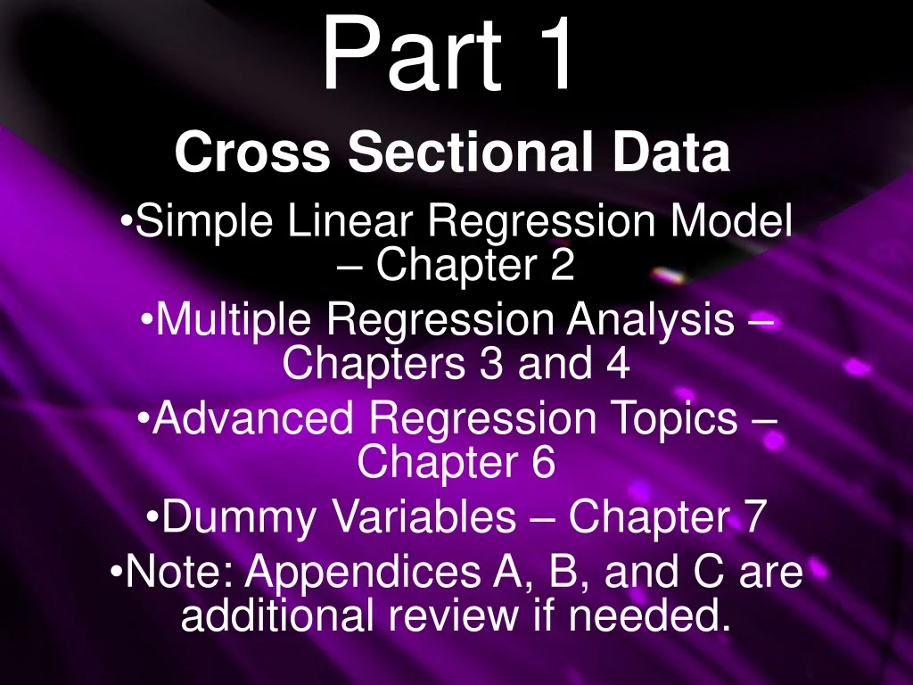
Part 1Cross Sectional Data Simple Linear Regression Model – Chapter 2 Multiple Regression Analysis – Chapters 3 and 4 Advanced Regression Topics – Chapter 6 Dummy Variables – Chapter 7 Note: Appendices A, B, and C are additional review if needed.
1. The Simple Regression Model 2.1 Definition of the Simple Regression Model 2.2 Deriving the Ordinary Least Squares Estimates 2.3 Properties of OLS on Any Sample of Data 2.4 Units of Measurement and Functional Form 2.5 Expected Values and Variances of the OLS Estimators 2.6 Regression through the Origin
2.1 The Simple Regression Model • Economics is built upon assumptions -assume people are utility maximizers -assume perfect information -assume we have a can opener • The Simple Regression Model is based on assumptions -more assumptions are required for more analysis -disproving assumptions leads to more complicated models
2.1 The Simple Regression Model • Recall the SIMPLE LINEAR REGRESION MODEL: -relates two variables (x and y) -also called the two-variable linear regression model or bivariate linear regression model y is the DEPENDENT or EXPLAINED variable x is the INDEPENDENT or EXPLANATORY variable y is a function of x
2.1 The Simple Regression Model • Recall the SIMPLE LINEAR REGRESION MODEL: u is the ERROR TERM or DISTURBANCE variable -u takes into account all factors other than x that affect y -u accounts for all “unobserved” impacts on y
2.1 The Simple Regression Model • Example of the SIMPLE LINEAR REGRESION MODEL: -taste depends on cooking time -taste is explained by cooking time -taste is a function of cooking time -u accounts for other factors affecting taste (cooking skill, ingredients available, random luck, differing taste buds, etc.)
2.1 The Simple Regression Model • The SRM shows how y changes: -for example, if B1=3, a 2 increase in x would cause a 6 unit change in y (2 x 3 = 6) -B1 is the SLOPE PARAMETER -B0 is the INTERCEPT PARAMETER or CONSTANT TERM -not always useful in analysis
2.1 The Simple Regression Model -note that this equation implies CONSTANT returns -the first x has the same impact on y as the 100th x -to avoid this we can include powers or change functional forms
2.1 The Simple Regression Model -in order to achieve a ceteris paribus analysis of x’s affect on y, we need assumptions of u’s relationship with x -in order to simplify our assumptions, we first assume that the average of u in the population is zero: -if Bo is included in the equation, it can always be modified to make (2.5) true -ie: if E(u)>0, simply increase B1
2.1 x, u and Dependence -we now need to assume that x and u are unrelated -if x and u are uncorrelated, u may still be correlated to functions such as x2 -we therefore need a stronger assumption: -the average value of u does not depend on x -second equality comes from (2.5) -called the ZERO CONDITIONAL MEAN ASSUMPTION
2.1 Example Take the regression: -where u takes into other factors of the applied paper, in particular length exceeding 10 pages -assumption (2.6) requires that a paper’s length does not depend on how good it is:
2.1 The Simple Regression Model • Conditional Expectations of (2.1) and (2.6) give us: -2.8 is called the POPULATION REGRESSION FUNCTION (PRF) -a one unit increase in x increases the expected value of y by B1 -B0+B1x is the systematic (explained) part of y -u is the unsystematic (unexplained) part of y
2.2 Deriving the OLS Estimates • In order to estimate B1 and B2, we need sample data -let {(x,y):i=1,….n} be a sample of n observations from the population -here yi is explained by xi with error term ui -y5 indicates the observation of y from the 5th data point -this regression plots a “best fit” line through our data points:
2.2 Deriving the OLS Estimates These OLS estimates create a straight line going through the “middle” of the estimates:
2.2 Deriving OLS Estimates In order to derive OLS, we first need assumptions. We must first assume that u has zero expected value: -Secondly, we must assume that the covariance between x and u is zero: -(2.10) and (2.11) can also be rewritten in terms of x and y as:
2.2 Deriving OLS Estimates -(2.12) and (2.13) imply restrictions on the joint probability of the POPULATION -given SAMPLE data, these equations become: -notice that the “hat” above B1 and B2 indicate we are now dealing with estimates -this is an example of “method of moments” estimation (see Section C for a discussion)
2.2 Deriving OLS Estimates Using summation properties, (2.14) simplifies to: Which can be rewritten as: Which is our OLS estimate for the intercept -therefore given data and an estimate of the slope, the estimated intercept can be determined
2.2 Deriving OLS Estimates By cancelling out 1/n and combining (2.17) and 2.15 we get: Which can be rewritten as:
2.2 Deriving OLS Estimates Recall the algebraic properties: And
2.2 Deriving OLS Estimates We can make the simple assumption that: Which essentially states that not all x’s are the same -ie: you didn’t do a survey where one question is “are you alive?” -This is essentially the key assumption needed to estimate B1hat
2.2 Deriving OLS Estimates All this gives us the OLS estimate for B1: Note that assumption (2.18) basically ensured the denominator is not zero. -also note that if x and y are positively (negatively) correlated, B1hat will be positive (negative)
2.2 Fitted Values OLS estimates of B1 and B2 give us a FITTED value for y when x=xi: -there is one fitted or predicted value of y for each observation of x -the predicted y’s can be greater than, less than or (rarely) equal to the actual y’s
2.2 Residuals The difference between the actual y values and the estimates is the ESTIMATED error, or residuals: -again, there is one residual for each observation -these residuals ARE NOT the same as the actual error term
2.2 Residuals The SUM OF SQUARED RESIDUALS can be expressed as: -if B1hat and B2hat are chosen to minimize (2.22), (2.14) and (2.15) are our FIRST ORDER CONDITIONS (FOC’S) and we are able to derive the same OLS estimates as above (2.17) and (2.19) -the term “OLS” comes from the fact that the square of the residuals is minimized
2.2 Why OLS? Why minimize the sum of the squared residuals? -Why not minimize the residuals themselves? -Why not minimize the cube of the residuals? -not all minimization techniques can be expressed as formulas -OLS has the advantage of deriving unbiasedness, consistency, and other important statistical properties.
2.2 Regression Line Our OLS regression supplies us with an OLS REGRESSION LINE: -note that as this is an equation of a line, there are no subscripts -B0hat is the predicted value of y when x=0 -not always a valid value -(2.23) is also called the SAMPLE REGRESSION FUNCTION (SRF) -different data sets will estimate different B’s
2.2 Deriving OLS Estimates The slope estimate: Shows the change in yhat when x changes, or alternatively, The change in x can be multiplied by B1hat to estimate the change in y.
2.2 Deriving OLS Estimates • Notes: 1) As the mathematics required to estimate OLS is difficult with more than a few data points, econometrics software (like Shazam) must be used. 2) A successful regression cannot conclude on causality, only comment on positive or negative relations between x and y 3) We often use the terminology “regress y on x” to estimate y=f(x)
2.3 Properties of OLS on Any Sample of Data • Review -Once again, simple algebraic properties are needed in order to build OLS’s foundation -OLS (B1hat and B2hat) can be used to calculate fitted values (yhat) -the residual (u) is the difference between the actual y values and the estimated y values (yhat)
2.3 Properties of OLS u=y-yhat Here yhat underpredicts y uhat y yhat
2.3 Properties of OLS 1) From the FOC of OLS (2.14), the sum of all residuals is zero: 2) Also from the FOC of OLS (2.15), the sample covariance between the regressors and the OLS residuals is zero: From 2.30, the left side of 2.31) is proportional to the required sample covariance
2.3 Properties of OLS 3) The point (xbar, ybar) is always on the OLS regression line (from 2.16): Further Algebraic Gymnastics: 1) From (2.30) we know that the sample average of the fitted y values equals the sample average of the actual y values:
2.3 Properties of OLS Further Algebraic Gymnastics: 2) 2.30 and 2.31 combine to prove that the covariance between yhat and uhat is zero Therefore OLS breaks down yi into two uncorrelated parts – a fitted value and a residual:
2.3 Sum of Squares From the idea of fitted and residual components, we can calculate the TOTAL SUM OF SQUARES (SST), the EXPLAINED SUM OF SQUARES (SSE) and the RESIDUAL SUM OF SQUARES (SSR)
2.3 Sum of Squares SST measures the sample variation in y. SSE measures the sample variation in yhat (the fitted component. SSR measures the sample variation in uhat (the residual component. These relate to each other as follows:
2.3 Proof of Squares The proof of (2.36) is as follows: Since we assumed that the covariance between residuals and fitted values is zero,
2.3 Properties of OLS on Any Sample of Data • Notes -An in-depth analysis of sample and inter-variable covariance is available in section C for individual study -SST, SSE and SSR have differing interpretations and labels for different econometric software. As such, it is always important to look up the base formula
2.3 Goodness of Fit -Once we’ve run a regression, the question is begged, “How well does x explain y.” -We can’t answer that yet, but we can ask, “How well does the OLS regression line fit the data?” -To measure this, we use R2, the COEFFICIENT OF DETERMINATION:
2.3 Goodness of Fit -”R2 is the ratio of the explained variation compared to the total variation” -”the fraction of the sample variation in y that is explained by x” -R2 always lies between zero and 1 -if R2=1, all actual points lie on the regression line (usually an error) -if R2≈0, the regression explains very little; OLS is a “poor fit”
2.3 Properties of OLS on Any Sample of Data • Notes -A low R2 is not uncommon in the social sciences, especially in cross-sectional analysis -econometric regressions should not be heavily judged due to a low R2 -for example, if R2=0.12, that means 12% of the variation is explained, which is better than the 0% before the regression
