Download
1 / 29
290 likes | 490 Vues
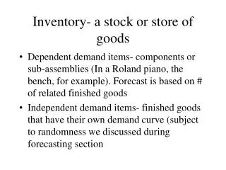
Inventory- a stock or store of goods. Dependent demand items- components or sub-assemblies (In a Roland piano, the bench, for example). Forecast is based on # of related finished goods

E N D
Inventory- a stock or store of goods • Dependent demand items- components or sub-assemblies (In a Roland piano, the bench, for example). Forecast is based on # of related finished goods • Independent demand items- finished goods that have their own demand curve (subject to randomness we discussed during forecasting section
Types of inventories- piano example • Raw materials & parts (e.g. piano keys) • Work In Process (keyboard assembly) • Finished Goods (keyboard, stand and bench) • Replacement items (keyboard cover handle) • In-transit inventory
Why keep inventory if it costs so much? • There are times in which the cost of keeping inventory is less than the benefits derived: • smooth production requirements as seen in Agg. Planning examples • decouple operations A distribution company wants to keep distributing even if the ship carrying the next shipment is late!
Why keep inventory if it costs so much? • To meet our stockout goals. Software is quick-decision purchase- many companies have 0% stockout strategies as a result (I.e. opportunity cost = 100%; inventory cost may equal 50%) • To capitalize on opportunities. If we have excess warehouse and staff capacity, we may save by buying a lot at a great price.
Ordering: quantity & timing Realities in the real world • Your order quantity may have to be done for political reasons (new product the president is behind- Edirol example) • We may not be able to affect the timing of orders. Distribution companies usually have to place 3 or even 6 month orders for highly technological products to smooth production planning. So fixed interval models are developed.
Counting Inventory • Periodic systems count physically at regular intervals and re-order when necessary. Your accounting audit will require this. • Perpetual systems (that count inventory as it changes in real time and re-ordering when we hit a reorder point) are almost universally used as the cost of computing has decreased. • Most companies combine use of both.
Adding math models to your tool kit • What is the lead time of your order (time between submission & receipt) • What is your holding cost (includes interest, insurance obsolescence, theft, wear, warehousing, etc.) • What is your ordering cost (including the cost of the transaction and receipt • What is your Shortage cost (opportunity)
What inventory do we evaluate? • Pareto principle tells us that 20% of our items will account for 80% of our orders/ supply requests • So, use the ABC system to classify value Item demand Unit Cost Annual $ value Class 1 10 50 500 2 100 1 100 3 75 300 22500 4 5 2500 12500 5 50 35 1750 6 130 50 6500
More on ABC System • Can be used to determine number of re-counts in physical counts (e.g. A’s get 3; B’s get 2; C’s get 1) • Can also be used to determine who does counts (A’s counted by controller, staff & warehouse; B’s by staff & warehouse; C’s by warehouse only)
The Inventory Cycle Profile of Inventory Level Over Time Q Usage rate Quantity on hand Reorder point Time Place order Place order Receive order Receive order Receive order Lead time
So we’ve evaluated the right inventory. Now let’s order. • EO Q Model minimizes the sum of holding and ordering costs by finding the optimal order quantity. • Assumptions: 1) one product at a time; 2) we’re confident in our annual demand forecast; 3) demand is even; 4) lead time is constant (management issue); 5) orders received in one delivery; 6) no qty discounts
Getting to EOQ: we’re balancing... • ANNUAL CARRYING COST = (Q/2)*H (Q= order quantity units; H- carrying cost/unit) • ANNUAL ORDERING COST = (D/Q)*S (D= annual unit demand; Q= order size; and S= ordering cost • calculus then gives us EO Q, the optimal order quantity
The Total-Cost Curve is U-Shaped Annual Cost Ordering Costs Order Quantity (Q) QO (optimal order quantity) Total cost = annual carrying cost + annual order cost Carrying Costs
Given that demand = 405/month • Carrying cost = $30/yr/unit Order Cost = $4/order • 1) EOQ= SQR(2*(405*12)*4)/30)= 36 • 2)What is average # of bags on hand? Q/2= 18 • 3) # of orders per year= (405*12)/36 =135 • 4) Carrying cost = (36/2)*30=540; ordering cost= (4860/36)*4=540 total cost = 540 +540 =1080 • **We need figures represented as annual costs.
Determining the economic run quantity of production • When company is producer and user, determines optimum production run size (since production usually happens faster than usage) • When we’re producing our own goods, assumes setup costs are the same as order costs in formula • so total cost = carrying cost +setup cost • TC = (Max. Inventory/2)*H + (D/Q)*S • Economic Run quantity = SQRRT(2DS/H)* SQRRT(p/(p-u)) where p=prod. Rate u=usage rate • cycle time =Q/u run time = Q/p
Quantity discounts if carrying costs are constant • Goal: minimize total cost, where TC = (Q/2)*H + (D/Q)*S + PD where P= unit price • Step 1: compute the common EOQ (if carrying cost is a constant $ figure, it won’t vary) • Step 2: compute total cost at EOQ and price breaks and compare
Quantity discounts if carrying costs are constant Assume: D5000,/yr h= $2/unit/yr s=$48 Units Price 1-399 $10 400-599 $9 600+ $8 • STEP 1: compute the common EOQ= SQR ((2DS)/H) = SQR((2*5000*48)/2)= 489.90 • STEP 2: compute the TC @ EOQ (490) = (Q/2)*H + (D/Q)*S + PD = (490/2)*2 + 5000/490)*48 + (9*5000) = $45980 (with rounding) • STEP 3: compare with TC at discount levels TC = (Q/2)*H + (D/Q)*S + PD TC @600 = (600/2)*2 + (5000/600)*48 + (8*5000)= 41000 • 600 is the optimum order quantity account for discounts
We know how much to order… now, when do we reorder? • ROP: predetermined inventory level of an item at which a reorder is placed. • Demand (d) and Lead TIME (LT) • ROP= d*LT • Example: Monthly demand is 400. Lead Time is two weeks (.50 months). ROP= 400 *.50 =200 • Reorder when inventory level reaches 200. • This model assumes static d and LT
What if demand or lead time is variable? • Then we add a safety stock to help us satisfy orders if demand is higher than expected. • Company policy: What is our service level? It is the number: 1- stock-out risk. “Our service level goal is 95%. In other words, there’s a 95% probability we won’t stock out.
Handling variability, 2 • We assume the variability is characterized by the normal distribution. • Turn to page 889. The shaded area under the curve represents the probability of us having inventory, given the variability in the average demand or average lead time. • So let’s say we have a service level goal of 95%. What is the Z score that characterizes 95% of the area under the normal curve? • About 1.645
When lead time is variable: • First example: LEAD TIME variable. • When lead time is variable, ROP= d* avgLT + z*d(LT) where d= demand rate; LT= lead time; LT=std. Dev. Of lead time • Get the z score (based on your service level goal) from the table as we saw on the last slide based on company’s stockout policy..
ROP= d* avgLT + z*d(LT) • Given: demand during lead time =400/day • Lead Time = 5 days, =2 acceptable stockout risk= 5% • STEP 1: get your Z score 1-.05 = .95 z (.95) =1.65 • STEP 2: plug in 400*5 + 1.65*400*2= 3320 • Reorder when inventory = 3320
If demand rate is variable: • ROP= avgd* LT + z* sqr.root of LT * (d) • assume: avg d =1000; d= 14; LT=4; company stockout policy = 10% risk. • Z score for .90 = 1.28 • 1000*4 + 1.28* 2 * 14= 4000+ 35.84= 4036 • in real world, d is derived by managers keeping careful records to determine it.
For next time • PROBLEMS (not questions) Ch 12 #s 1,6,13,19, • Page 587- know models 1,2,3, and 4a,b,c
Problem 1 Item Usage Unit Cost Value Class 4021 90 1400 126000 A 9402 300 12 3600 C 4066 30 700 21000 B 6500 150 20 3000 C 9280 10 1020 10200 C 4050 80 140 11200 C 6850 2000 10 20000 B 3010 400 20 8000 C 4400 5000 5 25000 B
Problem 6 • D=800/MO @ $10/UNIT S=$28 H= 35% OF UNIT COST/YR • D- 9600/YR H= $3.50/UNIT/YR • CURRENT TC = (q/2)*H + (D/Q)*S • CURRENT TC= (800/2)*3.50 + (9600/800)*28 =1736 • EOQ= square root of ((2DS)/H) • EOQ = SQR ((2*9600*28)/3.50) =SQR 153600 =391.91= 392 • TC at 392= (392/2 )*3.5 + (9600/392)*28=1371.71 • Cost savings =1736-1372=364
Problem 13: carrying costs are constant • D=18000 H= $0.60/yr S=$96 • STEP 1: Common EOQ= SQR ((2DS)/H) = SQR((2*18000*96)/.6)= 2400 • STEP 2: TC @2400 = (Q/2)*H + (D/Q)*S + PD =(2400/2)*0.60 + (18000/2400)*96 + (1.20*18000)=$23040 • TC @5000 = (5000/2)*0.60 + (18000/5000)*96 + (18000*1.15)=$22545.60 • TC@10000= (10000/2)*.60 + (18000/10000)*96 + 18000*1.10=22972.80 • 5000 is the optimum order quantity account for discounts
Problem 19, page 597 • see page 573, equation 12-12. The estimate of standard deviation of lead time demand is available, so you can use this simpler equation • Expected demand during LT = 300 Std dev of LT demand = 30 • a) Step 1 z=2.33 • a) step 2 300+(2.33*30)=69.9=370 • b) from a)--> 70 units • c)less safety stock is required because we’d be carrying an amount of inventory causing us to stock out more often.
Problem 23 • Hint: plot the information you do have under the equation, then solve for what you don’t have. • When the book says “the delivery time is normal” that means we’ve got a variable lead time problem. • When lead time is variable, ROP= d* avgLT + z*d(LT) where d= demand rate; LT= lead time; LT=std. Dev. Of lead time • 625= 85*6 + z*85*1.10 • solving for z, z=1.22 • from table on p. 883, that shows an 89% probability of supply, implying an 11% probability the supply will be exhausted.