Download
1 / 15
150 likes | 168 Vues
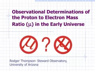
This study investigates the possible variations of the proton-to-electron mass ratio by analyzing microwave spectra of molecules. It explores the sensitivity coefficients, limits, and the potential implications of the observed variations. The results provide insights into fundamental constants and their time-variation at different redshifts.

E N D
Studying possible variations of proton-to-electron mass ratio with microwave spectra of molecules M G Kozlov, V V Flambaum, S A Levshakov, D Reimers, S G Porsev, and P Molaro
The constants which can be probed from astronomical spectra : • the fine-structure constant α=e2/ħc • The proton-to-electron mass ratio μ=mp/me • the nuclear gyromagnetic ratio gn Reported in the literature optical data concerning the relative variation of constants δμ/μandδα/αat redshifts z ~ 1–3are controversial at the level of a few ppm (1ppm = 10−6).
Sensitivity coefficients to the variation of fundamental constants The observed linewidth Γ in astrophysical spectra is usually determined by the Doppler broadening effect, i.e. where Δv is the velocity dispersion, c is the speed of light, and ω is the transition frequency. For extragalactic observations the typical values of Δv are about 1 – 10 km/s, which means that: The dimensionless sensitivity coefficients can be defined as:
If we observe two lines with different sensitivities and the same actual redshift, the apparent redshifts will differ by From the observation of one pair of lines it is impossible to distinguish between variation of different constants. Thus, we express difference in apparent redshift in terms of the variation of a following combination of fundamental constants: Obviouslywe should maximize either ΔKα, ΔKμ, or ΔKg. Usually sensitivity coefficients are calculated in the assumption, that atomic energy unit (27.2 eV) is independent of the fundamental constants. This assumption is only a matter of convenience, because only the differences in sensitivities are important.
Limits on variation of fundamental constants at redshifts z~1 (timescale of few Gyr) from microwave and infrared spectra
, where In 1996 Varshalovich & Potekhin compared apparent redshifts of rotational and optical lines to place following bound at z=1.9: In 2001 Murphy et al compared redshifts of 21 cm hydrogen line and a number of rotational lines for the object B0218+357 at the redshift z=0.68 to get the bound on variation of the product: Λ-doublet OH line from the same object B0218+357 was recently used to place very stringent bound on the variation of different combination of constants [Kanerar et al, 2005]: Finally, NH3 inversion line from B0218+357 allows to place limit on the variation of μ[Flambaum and Kozlov, 2007]:
The above limits are based on the analysis of different microwave lines of the same object B0218+357 at z=0.68. Simultaneous analysis of all these lines allow to have a complete experiment, i.e. to study all three fundamental constants relevant to atomic physics and place three model-independent limits on their time-variation: It would be extremely interesting to get new high precision data for this object for a dedicated and comprehensive analysis.
Using fine-structure lines to place bounds on time-variation at very high redshifts The redshift of the fine-structure [C II] 158 μm line is compared to that of the rotational CO line. Both lines are observed in emission for the quasars J1148+5251 and BR 1202-0725 with respective redshifts z=6.42 and z=4.69. The absence of the meaningful differences in apparent redshifts allowed to place bounds on the variation of the parameter Note that z=6.42 corresponds to the look-back time of approximately 12.9 Gyr, which constitutes 93% of the age of the Universe.
High precision data on variation of constants from microwave spectra of cold molecular clouds in our galaxy
Sun Galactic center. Schematic location of the Perseus molecular cloud, the Pipe Nebula, and the IRDCs in projection onto the Galactic plane.
Fig.1 Upper panel: C2S (21-10) versus NH3 (1,1) linewidths for cores in the Perseus molecular cloud from the total sample of Rosolowsky et al. (2008). Lower panel: Subsample of the best single-component profiles of C2S and NH3 selected from the full set.
Upper panel: Velocity offset ΔVCCS-NH3 versus the source radial velocity for points shown in the lower panel of Fig. 1. Lower panel: Same as the upper panel but for the points, which lie in allowed region between the lines.
Sample mean values (unweighted) ΔV , standard deviations σrms, robust M-estimates of the sample mean ΔVM, and the scale σM deduced from the original data and from the subsamples of molecular lines showing self-consistent linewidths.
Our final result from comparing redshifts of NH3 inversion line with rotational lines of other molecules for Perseus cloud, Pipe Nebulae, and IRDCs is: • This variation corresponds to the time intervals from 400 years for Pipe Nebulae to ~10000 years for IRDCs. Such time-variation contradicts both laboratory and extragalactic observations. • For the same reasons it can not be linked with gravitational potential. • It is possible to link this variation to the local matter density as suggested in some chamelion-type scalar field models.