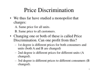

Price Discrimination: Capturing CS
E N D
Presentation Transcript
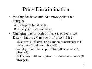
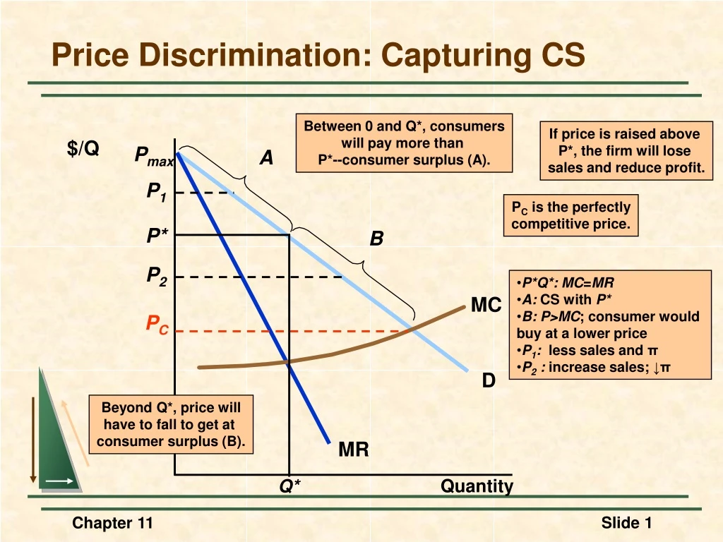
Between 0 and Q*, consumers will pay more than P*--consumer surplus (A). Pmax A P1 PC is the perfectly competitive price. P* B P2 MC PC D Beyond Q*, price will have to fall to get at consumer surplus (B). MR Q* Price Discrimination: Capturing CS If price is raised above P*, the firm will lose sales and reduce profit. $/Q • P*Q*:MC=MR • A: CS with P* • B:P>MC; consumer would • buy at a lower price • P1: less sales and π • P2 : increase sales; ↓π Quantity Chapter 11
Without price discrimination, output is Q* and price is P*. Variable profit is the area between the MC & MR (yellow). Consumer surplus is the area above P* and between 0 and Q* output. MC P* PC D = AR Output expands to Q** and price falls to PC where MC = MR = AR = D. Profits increase by the area above MC between old MR and D to output Q** (purple) MR Q* Q** First-Degree (Perfect) Price Discrimination $/Q Pmax Each consumer pays their reservation (maximum) price: Profits Increase Quantity Chapter 11
First Degree Price Discrimination • The model does demonstrate the potential profit (incentive) of using some degree of price discrimination. • Examples of imperfect price discrimination where the seller has some ability to segregate the market and charge different prices for the same product: • Lawyers, doctors, accountants • Car salesperson (15% profit margin) • Colleges and universities Chapter 11
Second-degree price discrimination is pricing according to quantity consumed--or in blocks. P1 Without discrimination: P = P0 and Q = Q0. With second-degree discrimination there are three prices P1, P2, and P3. (e.g. electric utilities) P0 P2 AC P3 MC D MR Q1 Q0 Q2 Q3 1st Block 2nd Block 3rd Block Second-Degree Price Discrimination $/Q Quantity
Third Degree Price Discrimination 1) Divides the market into two-groups. 2) Each group has its own demand function. 3) Most common type of price discrimination. • Examples: airlines, liquor, vegetables, discounts to students and senior citizens. 4) Feasible when the seller can separate his/her market into groups who have different price elasticities of demand (e.g. business air travelers versus vacation air travelers) Chapter 11
Third Degree Price Discrimination • Third Degree Price Discrimination • P1: price first group • P2: price second group • C(Qr) = total cost of QT = Q1 + Q2 • Profit ( ) = P1Q1 + P2Q2 - C(Qr) • Pricing: Charge higher price to group with a low demand elasticity. Chapter 11
Consumers are divided into two groups, with separate demand curves for each group. MRT = MR1 + MR2 D2 = AR2 MRT MR2 D1 = AR1 MR1 Third-Degree Price Discrimination $/Q Quantity Chapter 11
QT: MC = MRT • Group 1: P1Q1 ; more inelastic • Group 2: P2Q2; more elastic • MR1 = MR2 = MC • MC depends on QT P1 MC P2 Q1 Q2 QT Third-Degree Price Discrimination $/Q D2 = AR2 MRT MR2 D1 = AR1 MR1 Quantity Chapter 11
The Economics of Coupons and Rebates Price Discrimination • Those consumers who are more price elastic will tend to use the coupon/rebate more often when they purchase the product than those consumers with a less elastic demand. • Coupons and rebate programs allow firms to price discriminate. Chapter 11
Airline Fares • Differences in elasticities imply that some customers will pay a higher fare than others. • Business travelers have few choices and their demand is less elastic. • Casual travelers have choices and are more price sensitive. • The airlines separate the market by setting various restrictions on the tickets. • Less expensive: notice, stay over the weekend, no refund • Most expensive: no restrictions Chapter 11
Intertemporal Price Discrimination • Separating the Market With Time • Initial release of a product, the demand is inelastic • Book, Movie, Computer • Once this market has yielded a maximum profit, firms lower the price to appeal to a general market with a more elastic demand • Paper back books, Dollar Movies, Discount computers Chapter 11
Consumers are divided into groups over time. Initially, demand is less elastic resulting in a price of P1 . P1 Over time, demand becomes more elastic and price is reduced to appeal to the mass market. P2 D2 = AR2 AC = MC MR2 MR1 D1 = AR1 Q1 Q2 Intertemporal Price Discrimination $/Q Quantity Chapter 11
Peak-Load Pricing Peak-Load Pricing • Demand for some products may peak at particular times. E.g. Rush hour traffic, Electricity - late summer afternoons, Ski resorts on weekends • Capacity restraints will also increase MC. • Increased MR and MC would indicate a higher price. • MR is not equal for each market because one market does not impact the other market. Chapter 11
MC Peak-load price = P1 . P1 D1 = AR1 Off- load price = P2 . P2 MR1 D2 = AR2 MR2 Q2 Q1 Peak-Load Pricing $/Q Quantity Chapter 11
The Two-Part Tariff • The purchase of some products and services can be separated into two decisions, and therefore, two prices. • Examples: 1) Amusement Park: Pay to enter; Pay for rides and food within the park 2) Tennis Club: Pay to join; Pay to play 3) Rental of Mainframe Computers: Flat Fee; Processing Time 4) Safety Razor: Pay for razor; Pay for blades 5) Polaroid Film: Pay for the camera; Pay for the film Chapter 11
Usage price P* is set where MC = D. Entry price T* is equal to the entire consumer surplus. T* MC P* D Two-Part Tariff with a Single Consumer $/Q Quantity Chapter 11
The price, P*, will be greater than MC. Set T* at the surplus value of D2. T* A P* MC B C D1 = consumer 1 D2 = consumer 2 Q2 Q1 Two-Part Tariff with Two Consumers $/Q Quantity Chapter 11
The Two-Part Tariff • The Two-Part Tariff With Many Different Consumers • No exact way to determine P* and T*. • Must consider the trade-off between the entry fee T* and the use fee P*. • Low entry fee: High sales and falling profit with lower price and more entrants. • To find optimum combination, choose several combinations of P,T. • Choose the combination that maximizes profit. Chapter 11