Download
1 / 32
320 likes | 467 Vues
Effective Data Management Techniques - In the view of Stream data. 한국기술교육대학교 컴퓨터공학부 민준기. 1. Introduction. Stream data A growing number of applications generate streams of data Performance measurements in network monitoring and traffic management Call detail records in telecommunications

E N D
Effective Data Management Techniques- In the view of Stream data 한국기술교육대학교 컴퓨터공학부 민준기
1. Introduction • Stream data • A growing number of applications generate streams of data • Performance measurements in network monitoring and traffic management • Call detail records in telecommunications • Transactions in retail chains, ATM operations in banks • Log records generated by Web Servers • Sensor network data • Application characteristics • Massive volumes of data (several terabytes) • Records arrive at a rapid rate
1. Introduction • Traditional Data Processing • Stable Repository • Query the data many times • Stream Data Processing • Data arrivescontinuously • Data is processed withoutthe benefit of multiple passes • For stream data, users registerqueries priorly
2. Stream Data Management • Using RDBMS • Data streams as relation inserts, continuous queries as triggers or materialized views • Problems with this approach • Inserts are typically batched, high overhead • Expressiveness: simple conditions (triggers), no built-in notion of sequence (views) • No notion of approximation, resource allocation • Current systems don’t scale to large # of triggers
Stream Data Management System • STREAM[2] • Stanford • Telegraph[3] • Research project in UC Berkeley • AURORA[1] • MIT, Brown University, Brandeis University
STREAM • The Stanford Data Stream Management System • Data streams and stored relations • Declarative language for registering continuous queries CQL • Flexible query plans and execution strategies • Continuous monitoring and reoptimization subsystem • Aggressive sharing of state and computation among queries • Load-shedding by introducing approximation • Tools to monitor and manipulate query plan
STREAM Property Value Query Plan Join Selectivity Rate of tuple flow Legend Queue size
Telegraph-CQ • Research project in UC Berkeley • challenges • Adaptivity • eddies : tuple routing and operator scheduling • Shared continuous queries • amortizing query-processing costs by sharing the execution of multiple long-running queries • assumption of Telegraph’s design • very volatile, unpredictable environments • internet, sensor networks, wide-area federated S/W including peer-to-peer systems • performance is volatile • data rates change from moment to moment • services speed up, slow down, disappear and reappear over time • code behaves differently from moment to moment • data quality changes from moment to moment
Aurora • MIT, Brown University, Brandeis University • Features • Designed for Scalablility: • QoS-Driven Resource Management • Continuous and Historical Queries • Stream Storage Management
inputs outputs Storage Manager q1 q2 . . . s s qi m Buffer . . . . . . È È Persistent Store Catalog q1 q2 . . . qn … … … … … … Aurora Router Scheduler Box Processors QOS Monitor
Slide s s App App App QoS QoS QoS . . . . . . s s m . . . . . . . . . È m Tumble s m Aurora • Query Operators (Boxes) • Simple: FILTER, MAP • Binary: UNION, JOIN • Windowed: AGGREGATE, WSORT
Stream data Processing • The properties of stream data varies over time • Adaptiveness to generate an efficient plan with respect to the change of data properties is required • Improve the Performance of Stream Query Processing • Operator Scheduling • (NEXT WEEK) • Operator Ordering Query Optimization • Query Index
O1 O2 Queue Queue Queue Queue Stream Source O3 Operator Scheduling • Operator Scheduling • Select one operator among executable operators • Primitive scheduling • Eddy[4] • Chain[5] • Train[6] • Adaptive Scheduling[7]
Premitive Operator Scheduling • Process scheduling From OS • FIFO • Tuples are processed in the order that they arrive • Advantage • A consistent throughput • Round robin • Works by placing all runnable operators in a circular queue and allocating a fixed time slice to each • Advantage • Avoidance of starvation • Disadvantage • Does not adapt at all changing stream conditions • Large Queue size, poor output rate
R R (R.b < 15) (R.b < 15) (R.a > 10) (R.a > 10) R1 Eddy Eddy a b a b Ready Done Eddy: Telegraph-CQ[4] SELECT * FROM R WHERE R.a > 10 AND R.b < 15 Eddy : • lottery-type scheduler • Adapting to Long Running Queries • ready bit : indicate which operators can be applied to a tuple • done bit : indicate the operators to which a tuple has already been routed R2 R2 R1 R2 R2 R2 R1 R2 1 1 11 1 1 1 0 1 1 0 0 1 1 0 1 1 1 0 0
Chain[5] • STREAM • Purpose • minimize memory utilization • Assumption • Operator time t • Operator selectivity s
Chain[5] • Progress chart • m+1 operator pointers (t0,s0),(t1,s1), … (tm,sm) • ith operator oi takes ti-ti-1 time with si/si-1 selectivity
Chain[5] • For a point (t,s) where ti-1<= t< ti, the derivative with respect to the j th operator point where m>= j >= I, d(t,s,j) = -(sj-s)/tj-t • The steepest derivative D(t,s) = maxm>=j>=i d(t,s,j) • Steepest Descent Operator point • SDOP(t,s) = (tb,sb) where b = min{j | m>= j >=i and d(t,s,j) = D(t,s)} • Lower envelop • Connect the sequence of SDOPs • Chain • Schedule for a single time until the tuple that lies on the segment with the steepest slop in its lower envelope simulation. If there are multiple such tuples, select tuple which has the earliest arrival time • Chain is optimal with respect to memory utilization in single stream query (e.g., simple selections)
Chain[5] • Extending Chain to Joins • (t,s): Process time t and selectivity s • Average number of tuples in S : LS • Window size(time) :t’ • Input size : t’(LR+LS) • Output size : t’(LRaw(S) +LSaw(R)) • where aw(s) is the semijoin selectivity of stream R with sliding windows for S. • Time for run : t’(LRtR +LStS) • Where tx is the average time to process a tuple from stream X • Selectivity s for a join • (LRaw(S) +LSaw(R) )/ (LR+LS) • Processing time t for a join • (LRtR +LStS)/ LR+LS
Train[6] • Aurora data stream manager • Two-Level Scheduling • Which query to processing(i.e., select a query) • Static: application-at-a-time • Use various scheduling policies(e.g., round robin) • Dynamic: top-k spanner • QoS-driven • How selected query be processed • Operator scheduling
Train[6] • Operator scheduling • Traversing query tree • Three goals • Throughput • Latency • Memory requirement • QoS driven scheduling
Train[6] • Min-Cost(MC) • Optimize per-output-tuple processing cost • Traverse the query tree in post-order • b4-b5- b3-b2-b6-b1 • Assume • process cost per tuple p, a box call overhead o • A selectivity is 1 • Each operator has a queue with a single tuple Total cost: 15p+5o Average output latency: 12.5p+o
Train[6] • Min-Latency(ML) • Average latency of the output tuples can be reduced by producing initial output tuples as fast as possible • Output_cost(b): an estimate of the latency where D(b) is the set of operators downstream from b • Under the same condition of MC • b1-b2-b1-b6-b1-b4-b2-b1-b3-b2-b1-b5-b3-b2-b1 • Total cost: 15p+15o • Average latency: 7.17p+7.17o
Train[6] • Min-Memory(MM) • Maximize the consumption of data per unit time • Expected memory reduction rates for b where tsize(b) is the size of a tuple that reside on b’s input queue • Assume selectivity and cost: • b1=(0.9, 2), b2=(0.4,2) b3=(0.4, 3) b4=(1.0, 2) b5=(0.4,3), b6=(0.6,1) • All tuple size is 1 • Mem_rr: 0.05, 0.3, 0.5, 0, 0.2, 0.4 • Memory requirement • MM(36), MC(39), ML(40)
Train[6] • QoS driven scheduling • Each operator has priority= (utility, urgency) • Utility(b) = gradient(eol(b)) • eol(b) = latency(b) + cost(D(b)) Where D(b) is set of operators downstream from b and cost(D(b)) is an estimate of how long it will take to process Latency(b) is average latency of tuples in input queue • Urgency(b) = -est(b) where est(b) is an indication of how close a operator is to a critical point( a point where QoS changes sharply) Priority(b) = (utility(b), -est(b)) Select operator having the highest utility and choose one having minimum slack time.
Adaptive Scheduling[7] • WORCESTER Polytechnic institute • Master thesis • Raindrop system • No superior scheduling • Diverse QoS requirements • Output rate • Intermediate Query size • Tuple Delay • A single requirement for all queries
Adaptive Scheduling[7] • Update related statistics periodically. • Algorithm score • s is a mean of a statistics of a scheduler • H is mean for historical category H, (maxH-minH) is spread of values • decay reflects the unreliability of the score of algorithms that have not run for long time. (0 decay < 1) • time is elapse time since s was updated • If quantifier is maximize, zi = zi, otherwize, zi = 1-zi
Adaptive scheduling[7] • Roulette Wheel strategy • Assign each algorithm a slice of a ciurcular “roulette wheel” with size of the slice being proportional to the individual’s score. • Problem of this work • How to obtain not-runned schedulers’ statistics. • Inaccuracy of the score function • Not runned schedulers for long time 0.5 (due to decay) • Scheduler runs very well 0.5 (since s== H)
Reference • [1] D. Carney, U. Cetintemel, M. Cherniack, C. Convey, S. Lee,G. Seidman, M. Stonebraker, N. Tatbul, and S. Zdonik. Monitoring streams–a new class of data management applications. In Proc. 28th Intl. Conf. on Very Large Data Bases, Aug. 2002. • [2] A. Arasu, B. Babcock, S. Babu, M. Datar, K. Ito, R. Motwani, I. Nishizawa, U. Srivastava, D. Thomas, R. Varma, J. Widom, J., “Stream: The stanford stream data manager”, IEEE Data Engineering Bulletin, Vol 26, No 1, pp. 19-26, 2003. • [3]J. M. Hellerstein, M. J. Franklin, S. Chandrasekaran, A. Deshpande, K. Hildrum, S. Madden, V. Raman, V., M. A. Shah, “Adaptive query processing: Technology in evolution”, IEEE Data Engineering Bulletin, Vol 23, No 2, pp. 7-18, 2000. • [4] R. Avnur, J. M. Hellerstein, “Eddies: Continuously adaptive query processing”, In Proceedings of ACM SIGMOD Conference, pp. 261-272, 2000. • [5] Brain Babcock et.al, “Chain: Operator scheduling for Memory minimization in Data Stream Systems,” ACM SIGMOD 2003. • [6] Don Carney et.al, “Operator Scheduling in a Data Stream Manager”, VLDB 2003 • [7] B. Pielech, “Adaptive scheduling algorithm selection in a streaming query system,” Master thesis , Worcester polytechnic institute, 2004. • [8] N Tatbul, U Çetintemel, S Zdonik, M Cherniack, M Stonebraker, “Load shedding in a data stream manager”, VLDB 2003. • [9]. Babu, S., Motwani, R., Munagala, K., Nishizawa, I., Widom, J.: Adaptive ordering of pipelined stream filters. In: Proceedings of ACM SIGMOD Conference. (2004) 407–418 • [10] S. Madden, M.A. Shah, J.M. Hellerstein, V. Raman, “Continuously adaptive continuous queries over streams”, In Proceedings of ACM SIGMOD Conference, 2002. • [11] Jinwon Lee, Seungwoo Kang, Youngki Lee, SangJeong Lee, and Junehwa Song, "BMQ-Processor: A High-Performance Border Crossing Event Detection Framework for Large-scale Monitoring Applications", IEEE Transactions on Knowledge and Data Engineering (TKDE), Vol. 21, No. 2, pp 234-252, February 2009
Reference • [12] S. Madden et.al., “TAG: Aggregation Service for Ad-Hoc Sensor Networks”, OSDI, 2002 • [13] N. Shrivastava et.al., “Medians and Beyond: New Aggregation Techniques for Sensor Networks,” ACM Sensys 2004 • [14] N. Trigoni et.al., “Multi-Query Optimization for Sensor Networks” DCOSS 2005 • [15]N. Trigoni, et.al., "Routing and Processing Multiple Aggregate Queries in Sensor Networks,“ ACM SenSys, 2006. • [16] A. Deshpande et.al., "Model-Driven Data Acquisition in Sensor Networks,“ VLDB, 2004. • [17] D. Chu et.al., "Approximate Data Collection in Sensor Networks using Probabilistic Models,“ ICDE, 2006 • [18] D. Tulone et. al., “PAQ: Time Series Forecasting For Approximate Query Answering In Sensor Networks,” European Conf. Wireless Sensor Networks, 2006 • [19] A. Deligiannakis et.al., “Compressing Historical Information in Sensor Networks,” ACM SIGMOD 2004 • [20] A. Jain et.al., “Adaptive Stream Resource Management Using Kalman Filters,” ACM SIGMOD 2004 • [21] X. Yang et.al., “In-Network Execution of Monitoring Queries in Sensor Networks,” ACM SIGMOD 2007. • [22]M. Stern et.al., “Towards Efficient Processing of General-Purpose Joins in Sensor Networks,” ICDE 2009. • [23]A. Pandit et.al, “ Communication-Efficient Implementation of Range-Joins in Sensor Networks,” International Conference on Database Systems for Advanced Applications (DASFAA), 2006 • [24] H. Yu et.al, “In-Network Join Processing for Sensor Networks,” APWeb 2006. • [25] A. Coman et.al, “On Join Location in Sensor Networks,” MDM 2007. • [26] H.S. Lin, J.G. Lee, M.J. Lee, K.Y. Whang, I.Y. Song ,” Continuous Query Processing in Data Streams Using Duality of Data and Queries,” ACM SIGMOD 2006. • [27] B. Mozafari, C. Zaniolo, “Optimal Load Shedding with Aggregates and Mining Queries,” ICDE 2010.