Enhancing DNA Microarray Data Analysis with Support Feature Machine
This paper discusses a novel approach to analyzing DNA microarray data using Support Feature Machine (SFM), which builds on traditional Support Vector Machine (SVM) techniques. The main idea involves constructing an enhanced feature space that incorporates kernel features, improving classification results. The SFM approach emphasizes the generation of new features through linear projections and other mechanisms, facilitating better model performance on complex data structures. Comparisons between SFM and SVM demonstrate significant improvements in interpretation and results, making SFM a promising tool for bioinformatics applications.

Enhancing DNA Microarray Data Analysis with Support Feature Machine
E N D
Presentation Transcript
Support Feature Machine for DNA microarray data Tomasz Maszczyk and Włodzisław Duch Department of Informatics, Nicolaus Copernicus University, Toruń, Poland RSCTC 2010
Plan • Main idea • SFMvsSVM • Description of ourapproach • Results • Conclusions
Main idea • SVM – based on LDA with marginmaximization (goodgeneralization, control of complexity). • Non-lineardecisionborders – linearized by projectinginto high-dimensionalfeaturespace. • Covertheorem (increase P() data separable, flatteningdecisionborders). • Kernelmethods – newfeatureszi(x)=k(x,xi)constructedaround SV xi(vectorsclose to the decisionborders). • Insteadoriginalinputspacexi,SVM works in the space of kernelfeatures zi(x) called "the kernel space".
Main idea • Each SV ?= usefulfeature, optimal for data with particulardistributions, not work on parityorotherproblems with complexlogicalstructure. • For somehighly-non-separable problems localized linear projections may easily solve the problem. New useful features: random linear projections, principal components derived from data, or projection pursuit algorithms based on Quality of Projected Clusters (QPC). • Appropriate feature space ?= optimal solutions, learn from other models what interesting features they have discovered: prototypes, linear combinations, or fragments of branches in decision trees. • The final model - linear discrimination, Naive Bayes, nearest neighbor or a decision tree - is secondary, if appropriate space has been set up.
SFMvsSVM SFM generalize SVM explicitly building enhanced space that includes kernel features zi(x)=k(x,xi) together with any other features that may provide useful information. This approach has several advantages comparing to standard SVM: • With explicit representation of features interpretation of discriminant function is as simple as in any linear discrimination method. • Kernel-based SVM is equivalent to linear SVM in the explicitly constructed kernel space, therefore enhancing this space should lead to improvement of results.
SFMvsSVM • Kernels with various parameters may be used, including various degrees of localization, and the resulting discriminant may select global features, combining them with local features that handle exceptions. • Complexity of SVM is O(n2) due to the need of generating kernel matrix; SFM may select smaller number of kernel features from those vectors that project on overlapping regions in linear projections. • Many feature selection methods may be used to estimate usefulness of new features that define support feature space. • Many algorithms may be used in the support feature space to generate the final solution.
SFM SFM algorithm starts from std, followed by FS (Relief – onlypositiveweights). Such reduced, but still high dimensional data, is used to generate two types of new features: • Projections on m=Nc(Nc-1)/2 directions obtained by connecting pairs of centers wij=ci-cj, where ci is the mean of all vectors that belong to the Ci, i=1…Nc class. In high dimensional space such features ri(x)=wi·x help a lot (hist). FDA ?= betterdirections, moreexpensive. • Featuresbased on kernel features. Many types of kernels may be mixed together, including the same types of kernels with different parameters (only Gaussian kernels with fixed dispersion β) ti(x)=exp(-βΣ|xi-x|2). QPC on this feature space, generating additional orthogonal directions that are useful as new features. NQ=5 but CV shouldworksbetter.
Algorithm • Fix the Gaussian dispersion β and the number of QPC features NQ • Standardize dataset • Normalize the length of each vector to 1 • Perform Relief feature ranking, select only those with positive weights RWi > 0 • Calculate class centers ci, i=1...Nc, create m directions wij=ci-cj, i>j • Project all vectors on these directions rij(x) = wij·x (features rij) • Create kernel features ti(x)=exp(-βΣ|xi-x|2) • Create NQ QPC directions wi in the kernel space, adding QPC features si(x) = wi·x • Build linear model on the new feature space • Classify test data mapped into the new feature space
SFM - resume • In essence SFM requires construction of new features, followed by a simple linear model (LSVM) or any other learning model. • More attention to generation of features than to the sophisticated optimization algorithms or new classification methods. • Several parameters may be used to control the process of feature creation and selection but here they are fixed or set in an automatic way. Solutions are given in form of linear discriminant function and thus are easy to understand. • New features created in this way are based on those transformations of inputs that have been found interesting for some task, and thus have meaningful interpretation.
Results(SFM in extendedspaces) K=K(X,Xi) Z=WX H=[Z1,Z2]
Summary • SFM focused on generation of newfeatures, rather than improvement of optimization and classification algorithms. It may be regarded as an example of mixture of experts, where each expert is a simple model based on projection on some specific direction (random, or connecting clusters), localization of projected clusters (QPC), optimized directions (for example by FDA), or kernel methods based on similarity to reference vectors. For some data kernel-based features are most important, for other projections and restrictedprojections discover more interesting aspects. • Kernel-based SVM is equivalent to the use of kernel features combined with LSVM. Mixing different kernels and different types of features creates much better enhanced features space then a single-kernel solution. • Complex data may require decision borders of different complexity, and it is rather straightforward to introduce multiresolution in the presented algorithm, for example using different dispersion β for every ti, while in the standard SVM approach this is difficult to achieve.