Introducing ranked retrieval
Introducing ranked retrieval. Ch. 6. Ranked retrieval. Thus far, our queries have all been Boolean. Documents either match or don’t . Good for expert users with precise understanding of their needs and the collection.


Introducing ranked retrieval
E N D
Presentation Transcript
Ch. 6 Ranked retrieval • Thus far, our queries have all been Boolean. • Documents either match or don’t. • Good for expert users with precise understanding of their needs and the collection. • Also good for applications: Applications can easily consume 1000s of results. • Not good for the majority of users. • Most users incapable of writing Boolean queries (or they are, but they think it’s too much work). • Most users don’t want to wade through 1000s of results. • This is particularly true of web search.
Ch. 6 Problem with Boolean search:feast or famine • Boolean queries often result in either too few (≈0) or too many (1000s) results. • Query 1: “standard user dlink650” → 200,000 hits • Query 2: “standard user dlink 650 no card found” → 0 hits • It takes a lot of skill to come up with a query that produces a manageable number of hits. • AND gives too few; OR gives too many
Ranked retrieval models • Rather than a set of documents satisfying a query expression, in ranked retrieval models, the system returns an ordering over the (top) documents in the collection with respect to a query • Free text queries: Rather than a query language of operators and expressions, the user’s query is just one or more words in a human language • In principle, there are two separate choices here, but in practice, ranked retrieval models have normally been associated with free text queries and vice versa
Ch. 6 Feast or famine: not a problem in ranked retrieval • When a system produces a ranked result set, large result sets are not an issue • Indeed, the size of the result set is not an issue • We just show the top k ( ≈ 10) results • We don’t overwhelm the user • Premise: the ranking algorithm works
Ch. 6 Scoring as the basis of ranked retrieval • We wish to return in order the documents most likely to be useful to the searcher • How can we rank-order the documents in the collection with respect to a query? • Assign a score – say in [0, 1] – to each document • This score measures how well document and query “match”.
Ch. 6 Query-document matching scores • We need a way of assigning a score to a query/document pair • Let’s start with a one-term query • If the query term does not occur in the document: score should be 0 • The more frequent the query term in the document, the higher the score (should be) • We will look at a number of alternatives for this
Ch. 6 Take 1: Jaccard coefficient • A commonly used measure of overlap of two sets A and B is the Jaccard coefficient • jaccard(A,B) = |A ∩ B| / |A ∪ B| • jaccard(A,A) = 1 • jaccard(A,B) = 0if A ∩ B = 0 • A and Bdon’t have to be the same size. • Always assigns a number between 0 and 1.
Ch. 6 Jaccard coefficient: Scoring example • What is the query-document match score that the Jaccard coefficient computes for each of the two documents below? • Query: ides of march • Document 1: caesar died in march • Document 2: the long march
Ch. 6 Issues with Jaccard for scoring • It doesn’t consider term frequency (how many times a term occurs in a document) • Rare terms in a collection are more informative than frequent terms • Jaccard doesn’t consider this information • We need a more sophisticated way of normalizing for length • Later in this lecture, we’ll use . . . instead of |A ∩ B|/|A ∪ B| (Jaccard) for length normalization.
Sec. 6.2 Recall: Binary term-document incidence matrix Each document is represented by a binary vector ∈ {0,1}|V|
Sec. 6.2 Term-document count matrices • Consider the number of occurrences of a term in a document: • Each document is a count vector in ℕ|V|: a column below
Bag of words model • Vector representation doesn’t consider the ordering of words in a document • John is quicker than Maryand Mary is quicker than John have the same vectors • This is called the bag of wordsmodel. • In a sense, this is a step back: The positional index was able to distinguish these two documents • We will look at “recovering” positional information later on • For now: bag of words model
Term frequency tf • The term frequency tft,d of term t in document d is defined as the number of times that t occurs in d. • We want to use tf when computing query-document match scores. But how? • Raw term frequency is not what we want: • A document with 10 occurrences of the term is more relevant than a document with 1 occurrence of the term. • But not 10 times more relevant. • Relevance does not increase proportionally with term frequency. NB: frequency = count in IR
Sec. 6.2 Log-frequency weighting • The log frequency weight of term t in d is • Score for a document-query pair: sum over terms t in both q and d: • score • The score is 0 if none of the query terms is present in the document.
Sec. 6.2.1 Document frequency • Rare terms are more informative than frequent terms • Recall stop words • Consider a term in the query that is rare in the collection (e.g., arachnocentric) • A document containing this term is very likely to be relevant to the query arachnocentric • → We want a high weight for rare terms like arachnocentric.
Sec. 6.2.1 Document frequency, continued • Frequent terms are less informative than rare terms • Consider a query term that is frequent in the collection (e.g., high, increase, line) • A document containing such a term is more likely to be relevant than a document that doesn’t • But it’s not a sure indicator of relevance. • → For frequent terms, we want positive weights for words like high, increase, and line • But lower weights than for rare terms. • We will use document frequency (df) to capture this.
Sec. 6.2.1 idf weight • dft is the document frequency of t: the number of documents that contain t • dft is an inverse measure of the informativeness of t • dft N • We define the idf (inverse document frequency) of t by • We use log (N/dft) instead of N/dft to “dampen” the effect of idf. Will turn out the base of the log is immaterial.
Sec. 6.2.1 idf example, suppose N = 1 million There is one idf value for each term t in a collection.
Effect of idf on ranking • Question: Does idf have an effect on ranking for one-term queries, like • iPhone
Effect of idf on ranking • Question: Does idf have an effect on ranking for one-term queries, like • iPhone • idf has no effect on ranking one term queries • idf affects the ranking of documents for queries with at least two terms • For the query capricious person, idf weighting makes occurrences of capricious count for much more in the final document ranking than occurrences of person.
Sec. 6.2.1 Collection vs. Document frequency • The collection frequency of t is the number of occurrences of t in the collection, counting multiple occurrences. • Example: • Which word is a better search term (and should get a higher weight)?
Sec. 6.2.2 tf-idf weighting • The tf-idf weight of a term is the product of its tf weight and its idf weight. • Best known weighting scheme in information retrieval • Note: the “-” in tf-idf is a hyphen, not a minus sign! • Alternative names: tf.idf, tf x idf • Increases with the number of occurrences within a document • Increases with the rarity of the term in the collection
Sec. 6.2.2 Final ranking of documents for a query
Sec. 6.3 Binary → count → weight matrix Each document is now represented by a real-valued vector of tf-idf weights ∈ R|V|
Sec. 6.3 Documents as vectors • Now we have a |V|-dimensional vector space • Terms are axes of the space • Documents are points or vectors in this space • Very high-dimensional: tens of millions of dimensions when you apply this to a web search engine • These are very sparse vectors – most entries are zero
Sec. 6.3 Queries as vectors • Key idea 1:Do the same for queries: represent them as vectors in the space • Key idea 2:Rank documents according to their proximity to the query in this space • proximity = similarity of vectors • proximity ≈ inverse of distance • Recall: We do this because we want to get away from the you’re-either-in-or-out Boolean model • Instead: rank more relevant documents higher than less relevant documents
Sec. 6.3 Formalizing vector space proximity • First cut: distance between two points • ( = distance between the end points of the two vectors) • Euclidean distance? • Euclidean distance is a bad idea . . . • . . . because Euclidean distance is large for vectors of different lengths.
Sec. 6.3 Why distance is a bad idea The Euclidean distance between q and d2 is large even though the distribution of terms in the query qand the distribution of terms in the document d2 are very similar.
Sec. 6.3 Use angle instead of distance • Thought experiment: take a document d and append it to itself. Call this document d′. • “Semantically” d and d′ have the same content • The Euclidean distance between the two documents can be quite large • The angle between the two documents is 0, corresponding to maximal similarity. • Key idea: Rank documents according to angle with query.
Sec. 6.3 From angles to cosines • The following two notions are equivalent. • Rank documents in decreasing order of the angle between query and document • Rank documents in increasingorder of cosine(query,document) • Cosine is a monotonically decreasing function for the interval [0o, 180o]
Sec. 6.3 From angles to cosines • But how – and why – should we be computing cosines?
Sec. 6.3 Length normalization • A vector can be (length-) normalized by dividing each of its components by its length – for this we use the L2 norm: • Dividing a vector by its L2 norm makes it a unit (length) vector (on surface of unit hypersphere) • Effect on the two documents d and d′ (d appended to itself) from earlier slide: they have identical vectors after length-normalization. • Long and short documents now have comparable weights
Sec. 6.3 cosine(query,document) Dot product Unit vectors qi is the tf-idf weight of term i in the query di is the tf-idf weight of term i in the document cos(q,d) is the cosine similarity of q and d … or, equivalently, the cosine of the angle between q and d.
Cosine for length-normalized vectors • For length-normalized vectors, cosine similarity is simply the dot product (or scalar product): for q, d length-normalized.
Sec. 6.3 Cosine similarity amongst 3 documents How similar are the novels SaS: Sense and Sensibility PaP: Pride and Prejudice, and WH: Wuthering Heights? Term frequencies (counts) Note: To simplify this example, we don’t do idf weighting.
Sec. 6.3 3 documents example contd. Log frequency weighting After length normalization cos(SaS,PaP) ≈ 0.789 × 0.832 + 0.515 × 0.555 + 0.335 × 0.0 + 0.0 × 0.0 ≈ 0.94 cos(SaS,WH) ≈ 0.79 cos(PaP,WH) ≈ 0.69 Why do we have cos(SaS,PaP) > cos(SAS,WH)?
Calculating tf-idf cosine scores in an IR system