Objectives (BPS chapter 10)
Objectives (BPS chapter 10). Introducing probability The idea of probability Probability models Probability rules Discrete sample space Continuous sample space Random variables. Randomness and probability.

Objectives (BPS chapter 10)
E N D
Presentation Transcript
Objectives (BPS chapter 10) Introducing probability • The idea of probability • Probability models • Probability rules • Discrete sample space • Continuous sample space • Random variables
Randomness and probability A phenomenon is random if individual outcomes are uncertain, but there is nonetheless a regular distribution of outcomes in a large number of repetitions. The probability of any outcome of a random phenomenon can be defined as the proportion of times the outcome would occur in a very long series of repetitions.
The result of any single coin toss is random. But the result over many tosses is predictable, as long as the trials are independent (i.e., the outcome of a new coin toss is not influenced by the result of the previous toss). Coin toss The probability of heads is 0.5 = the proportion of times you get heads in many repeated trials. First series of tosses Second series
Two events are independent if the probability that one event occurs on any given trial of an experiment is not affected or changed by the occurrence of the other event. When are trials not independent? Imagine that these coins were spread out so that half were heads up and half were tails up. Close your eyes and pick one. The probability of it being heads is 0.5. However, if you don’t put it back in the pile, the probability of picking up another coin and having it be heads is now less than 0.5. The trials are independent only when you put the coin back each time. It is called sampling with replacement.
Probability models • Probability models mathematically describe the outcome of random processes. They consist of two parts: • 1) S = Sample Space: This is a set, or list, of all possible outcomes of a random process. An event is a subset of the sample space. • 2) A probability for each possible event in the sample space S. Example: Probability Model for a Coin Toss S = {Head, Tail} Probability of heads = 0.5 Probability of tails = 0.5
H - HHH H M - HHM H S = {HHH, HHM, HMH, HMM, MHH, MHM, MMH, MMM } Note: 8 elements, 23 H - HMH M M - HMM M … … Sample space Important: It’s the question that determines the sample space. A. A basketball player shoots three free throws. What are the possible sequences of hits (H) and misses (M)? B. A basketball player shoots three free throws. What is the number of baskets made? S = {0, 1, 2, 3} C. A nutrition researcher feeds a new diet to a young male white rat. What are the possible outcomes of weight gain (in grams)? S = [0, ∞] = (all numbers ≥ 0)
2) The probability of the complete sample space must equal 1. P(sample space) = 1 P(head) + P(tail) = 0.5 + 0.5 = 1 3) The probability of an event not occurring is 1 minus the probability that does occur. P(A) = 1 – P(not A) P(tail) = 1 – P(head) = 0.5 Coin Toss Example: S = {Head, Tail} Probability of heads = 0.5 Probability of tails = 0.5 Probability rules 1) Probabilities range from 0 (no chance of the event) to1 (the event has to happen). For any event A, 0 ≤ P(A) ≤ 1 Probability of getting a head = 0.5 We write this as: P(head) = 0.5 P(neither head nor tail) = 0 P(getting either a head or a tail) = 1
Probability rules (cont'd) A and B disjoint 4) Two events A and B are disjoint if they have no outcomes in common and can never happen together. The probability that A or B occurs is the sum of their individual probabilities. P(A or B) = “P(A U B)” = P(A) + P(B) This is the addition rule for disjoint events. A and B not disjoint Example:If you flip two coins and the first flip does not affect the second flip, S = {HH, HT, TH, TT}. The probability of each of these events is 1/4, or 0.25. The probability that you obtain “only heads or only tails” is:P(HH or TT) = P(HH) + P(TT) = 0.25 + 0.25 = 0.50
Discrete sample space Discrete sample spaces deal with data that can take on only certain values. These values are often integers or whole numbers. • Dice are good examples of finite sample spaces. Finite means that there is a limited number of outcomes. • Throwing 1 die: • S = {1, 2, 3, 4, 5, 6}, and the probability of each event = 1/6. Note: Discrete data contrast with continuous data that can take on any one of an infinite number of possible values over an interval.
In some situations, we define an event as a combination of outcomes. In that case, the probabilities need to be calculated from our knowledge of the probabilities of the simpler events. Example: You toss two dice. What is the probability of the outcomes summing to five? This isS: {(1,1), (1,2), (1,3), ……etc.} There are 36 possible outcomes in S, all equally likely (given fair dice). Thus, the probability of any one of them is 1/36. P(the roll of two dice sums to 5) = P(1,4) + P(2,3) + P(3,2) + P(4,1) = 4 * 1/36 = 1/9 = 0.111
The gambling industry relies on probability distributions to calculate the odds of winning. The rewards are then fixed precisely so that, on average, players lose and the house wins. The industry is very tough on so-called “cheaters” because their probability to win exceeds that of the house. Remember that it is a business, and therefore it has to be profitable.
Give the sample space and probabilities of each event in the following cases: • A couple wants three children. What are the arrangements of boys (B) and girls (G)? Genetics tells us that the probability that a baby is a boy or a girl is the same, 0.5. → Sample space: {BBB, BBG, BGB, GBB, GGB, GBG, BGG, GGG} → All eight outcomes in the sample space are equally likely. → The probability of each is thus 1/8. • A couple wants three children. What are the numbers of girls (X) they could have? The same genetic laws apply. We can use the probabilities above to calculate the probability for each possible number of girls. → Sample space {0, 1, 2, 3}→P(X = 0) = P(BBB) = 1/8→P(X = 1) = P(BBG or BGB or GBB) = P(BBG) + P(BGB) + P(GBB) = 3/8
Continuous sample space • Continuoussample spaces contain an infinite number of events. They typically are intervals of possible, continuously-distributed outcomes. • Example: There is an infinity of numbers between 0 and 1 (e.g., 0.001, 0.4, 0.0063876). • S = {interval containing all numbers between 0 and 1} • How do we assign probabilities to events in an infinite sample space? • We use density curves and compute probabilities for intervals. This is a uniform density curve. There are a lot of other types of density curves. The probability of the uniformly-distributed variable Y to be within 0.3 and 0.7 is the area under the density curve corresponding to that interval. Thus: P(0.3 ≤ y ≤ 0.7) = (0.7 − 0.3)*1 = 0.4 y
Probability distribution for a continuous random variable % individuals with X such that x1 < X < x2 The shaded area under the density curve shows the proportion, or percent, of individuals in the population with values of X between x1 and x2. Because the probability of drawing one individual atrandom depends on the frequency of this type of individual in the population, the probability is also the shaded area under the curve.
Intervals The probability of a single event is meaningless for a continuous sample space. Only intervals can have a non-zero probability, represented by the area under the density curve for that interval. The probability of a single event is zero: P(y = 1) = (1 − 1)*1 = 0 The probability of an interval is the same whether boundary values are included or excluded: P(0 ≤ y ≤ 0.5) = (0.5 − 0)*1 = 0.5 P(0 < y < 0.5) = (0.5 − 0)*1 = 0.5 P(0 ≤ y < 0.5) = (0.5 − 0)*1 = 0.5 Height = 1 y P(y < 0.5 or y > 0.8) = P(y < 0.5) + P(y > 0.8) = 1 −P(0.5 < y < 0.8) = 0.7
0.125 0.5 0.25 0.125 0 2 0.5 1 1.5 We generate two random numbers between 0 and 1 and take Y to be their sum. Y can take any value between 0 and 2. The density curve for Y is: Height = 1. We know this because the base = 2, and the area under the curve has to equal 1 by definition. The area of a this triangle is ½ (base*height). Y 0 1 2 What is the probability that Y is < 1? What is the probability that Y < 0.5?
Normal probability distribution A variable whose value is a number resulting from a random process is a random variable. The probability distribution of many random variables is the normal distribution. It shows what values the random variable can take and is used to assign probabilities to those values. Example: Probability distribution of women’s heights. Here, since we chose a woman randomly, her height, X, is a random variable. To calculate probabilities with the normal distribution, we will standardize the random variable (z-score) and use Table A.
N(64.5, 2.5) N(0,1) → Standardized height (no units) Reminder: standardizing N (m,s) We standardize normal data by calculating z-scores so that any Normal curve N(m,s) can be transformed into the standard Normal curve N(0,1).
Previously, we wanted to calculate the proportion of individuals in the population with a given characteristic. Distribution of women’s heights ≈ N (µ, ) = N (64.5, 2.5) Example: What's the proportion of women with a height between 57" and 72"? That’s within ± 3 standard deviations s of the mean m, thus that proportion is roughly 99.7%. Since about 99.7% of all women have heights between 57" and 72", the chance of picking one woman at random with a height in that range is also about 99.7%.
As before, we calculate the z-scores for 68 and 70. For x = 68", For x = 70", What is the probability, if we pick one woman at random, that her height will be some value X? For instance, between 68” and 70” P(68 < X < 70)? Because the woman is selected at random, X is a random variable. N(µ, s) = N(64.5, 2.5) 0.9192 0.9861 The area under the curve for the interval [68" to 70"] is 0.9861 − 0.9192 = 0.0669. Thus, the probability that a randomly chosen woman falls into this range is 6.69%. P(68 < X < 70) = 6.69%
s = 0.2 oz. Lowest2% x = 8 oz. m = ? Inverse problem: Your favorite chocolate bar is dark chocolate with whole hazelnuts. The weight on the wrapping indicates 8 oz. Whole hazelnuts vary in weight, so how can they guarantee you 8 oz. of your favorite treat? You are a bit skeptical... To avoid customer complaints and lawsuits, the manufacturer makes sure that 98% of all chocolate bars weight 8 oz. or more. The manufacturing process is roughly normal and has a known variability s = 0.2 oz. How should they calibrate the machines to produce bars with a mean msuch that P(x < 8 oz.) = 2%?
s = 0.2 oz. Lowest2% x = 8 oz. m = ? How should they calibrate the machines to produce bars with a mean m such that P(x < 8 oz.) = 2%? Here, we know the area under the density curve (2% = 0.02) and we know x (8 oz.). We want m . In Table A we find that the z for a left area of 0.02 is roughly z = 2.05. Thus, your favorite chocolate bar weighs, on average, 8.41 oz. Excellent!!!
Meaning of a probability We have several ways of defining a probability, and this has consequences on its intuitive meaning. • Theoretical probability From understanding the phenomenon and symmetries in the problem • Example: Six-sided fair die: Each side has the same chance of turning up; therefore, each has a probability 1/6. • Example: Genetic laws of inheritance based on meiosis process. • Empirical probability From our knowledge of numerous similar past events • Mendel discovered the probabilities of inheritance of a given trait from experiments on peas, without knowing about genes or DNA. • Example: Predicting the weather: A 30% chance of rain today means that it rained on 30% of all days with similar atmospheric conditions.