Objectives (BPS chapter 19)
Objectives (BPS chapter 19). Comparing two population means Two-sample t procedures Examples of two-sample t procedures Using technology Robustness again Details of the t approximation Avoid the pooled two-sample t procedures Avoid inference about standard deviations

Objectives (BPS chapter 19)
E N D
Presentation Transcript
Objectives (BPS chapter 19) Comparing two population means • Two-sample t procedures • Examples of two-sample t procedures • Using technology • Robustness again • Details of the t approximation • Avoid the pooled two-sample t procedures • Avoid inference about standard deviations • The F test for comparing two standard deviations
Conditions for inference comparing two means We have two independent SRSs (simple random samples) coming from two distinct populations (like men vs. women) with (m1,s1) and (m2,s2) unknown. Both populations should be Normally distributed. However, in practice, it is enough that the two distributions have similar shapes and that the sample data contain no strong outliers.
C mm −t* t* Two sample t-confidence interval Because we have two independent samples we use the difference between both sample averages ( 1 −2) to estimate (m1−m2). Practical use of t: t* • C is the area between −t* and t*. • We find t* in the line of Table C for df = smallest (n1−1; n2−1) and the column for confidence level C. • The margin of error m is:
Can directed reading activities in the classroom help improve reading ability? A class of 21 third-graders participates in these activities for 8 weeks while a control classroom of 23 third-graders follows the same curriculum without the activities. After the 8 weeks, all children take a reading test (scores in table). 95% confidence interval for (µ1 − µ2), with df = 20 conservatively t* = 2.086: With 95% confidence, (mu1 – mu2) falls within 9.96 ± 8.99 or 1.0 to 18.9.
Two-sample t-test The null hypothesis is that both population means m1 and m2 are equal, thus their difference is equal to zero. H0: m1 = m2 <=> m1−m2 = 0 with either a one-sided or a two-sided alternative hypothesis. We find how many standard errors (SE) away from (m1−m2) is ( 1 − 2) by standardizing with t: Because in a two-sample test H0poses (m1 - m2) = 0, we simply use with df = smallest(n1 − 1,n2 − 1)
Does smoking damage the lungs of children exposed to parental smoking? Forced Vital Capacity (FVC) is the volume (in milliliters) of air that an individual can exhale in 6 seconds. FVC was obtained for a sample of children not exposed to parental smoking and a group of children exposed to parental smoking. We want to know whether parental smoking decreases children’s lung capacity as measured by the FVC test. Is the mean FVC lower in the population of children exposed to parental smoking?
H0: msmoke = mno <=> (msmoke−mno) = 0 Ha: msmoke < mno <=> (msmoke−mno) < 0 (one sided) The difference in sample averages follows approximately the t distribution: We calculate the t statistic: In Table C, for df 29 we find:|t| > 3.659 => p < 0.0005 (one-sided) It’s a very significant difference, we reject H0. Lung capacity is significantly impaired in children of smoking parents.
Robustness The two-sample statistic is the most robust when both sample sizes are equal and both sample distributions are similar. But even when we deviate from this, two-sample tests tend to remain quite robust. As a guideline, a combined sample size (n1 + n2) of 40 or more will allow you to work even with the most skewed distributions.
Comparing vitamin content of bread, immediately after baking versus 3 days later (the same loaves are used on day one and 3 days later). Comparing vitamin content of bread, immediately after baking versus 3 days later (tests made on independent loaves). Average fuel efficiency for 2005 vehicles is 21 miles per gallon. Is average fuel efficiency higher in the new generation “green vehicles?” Is blood pressure altered by use of an oral contraceptive? Comparing a group of women not using an oral contraceptive with a group taking it. Review insurance records for dollar amount paid after fire damage in houses equipped with a fire extinguisher versus houses without one. Was there a difference in the average dollar amount paid? Which type of test? One sample, paired samples, two samples?
Comparing two standard deviations It is also possible to compare two population standard deviations σ1 and σ2 by comparing the standard deviations of two SRSs. However, the procedures are not robust at all against deviations from normality. When s12and s22are sample variances from independent SRSs of sizesn1 and n2 drawn from normal populations, the F-statisticF =s12/ s22 has the F distribution with n1 −1 and n2 −1 degrees of freedom whenH0: σ1 = σ2 is true. The F-value is then compared with critical values from Table D for the P-value with a one-sided alternative; this P-value is doubled for a two-sided alternative.

