Shifting Supply, Demand, and Equilibrium
270 likes | 560 Vues
Shifting Supply, Demand, and Equilibrium. With Graphing Applications. Reasons for Changes in Demand. Assume that Demand Curve B represents the baseline (original) consumption of beef in the month of May. For each of the following scenarios, decide:

Shifting Supply, Demand, and Equilibrium
E N D
Presentation Transcript
Shifting Supply, Demand, and Equilibrium With Graphing Applications
Reasons for Changes in Demand Assume that Demand Curve B represents the baseline (original) consumption of beef in the month of May. For each of the following scenarios, decide: Will this event cause a shift in the demand curve? If so, will the demand increase or decrease? Which demand curve likely represents the new demand for beef?
Scenario 1: Beef Prices Expected to Rise This is a Change in Consumer Expectations. Since people are expecting a rise in prices in the future, they will choose to buy now. As a result, the demand curve for beef will shift to the right to Demand Curve C – representing the increase in demand.
Scenario 2: Significant Number of Immigrants Arrive This is a Change in the Number of Consumers. More mouths to feed means more people buying beef. As a result, the demand curve for beef will shift to the right to Demand Curve C – representing the increase in demand.
Scenario 3: Pork Prices Drop This is a Change in the Price of a Substitute Good. Because it has become less expensive, more people are buying pork instead of beef. As a result, the demand curve for beef will shift to the left to Demand Curve A – representing the decrease in demand.
Scenario 4: Surgeon General Warns that Eating Beef is Hazardous to Health This is a Change in Consumer Tastes. Because of the Surgeon General’s warning, health-conscious consumers will choose alternative foods. As a result, the demand curve for beef will shift to the left to Demand Curve A – representing the decrease in demand.
Scenario 5: Beef Prices Fall This is movement along the original curve, so there is no shift. The graph of beef demand stays at Demand Curve B and the point of actual quantity demanded on that line moves.
Scenario 6: Real Income Drops for 3rd Month This is a Change in Income. With their income decreasing, people are choosing to buy less and save more. Alternatively, they might purchase less expensive alternatives to beef. As a result, the demand curve for beef will shift to the left to Demand Curve A – representing the decrease in demand.
Scenario 7: Charcoal Shortage Threatens Holiday Cookouts This is a Change in the Price of a Complimentary Product. Because charcoal is in short supply, it’s likely to be very expensive. Since charcoal grilling is a preferred way of preparing beef on a holiday weekend, people will likely buy less beef. As a result, the demand curve for beef will shift to the left to Demand Curve A – representing the decrease in demand.
Scenario 8: New Burger Restaurant Sweeps the Nation This is a Change in Consumer Tastes. Since this new burger place is so popular, they are buying beef to meet the number of customer orders. As a result, the demand curve will shift to the right to Demand Curve C – representing the increase in demand.
Reasons for Changes in Supply Assume that Supply Curve B represents the baseline (original) supply of foreign and domestic cars. For each of the following scenarios, decide: Will this event cause a shift in the supply curve? If so, will the supply increase or decrease? Which supply curve likely represents the new supply for foreign and domestic cars?
Scenario 1: Auto Workers’ Union Agrees to Wage Cuts This is a Change in Input Prices. Because they’ll be able to pay their workers less, this reduces the unit cost to produce cars – so suppliers have an impetus to produce more. As a result, the supply curve will shift to the right to Supply Curve C – representing the increase in supply.
Scenario 2: New Robot Technology Increases Efficiency This is a Change in Technology (which is also an Input). Because they’ll be able to produce cars more efficiency, this reduces the unit cost to produce cars – so suppliers have an impetus to produce more. As a result, the supply curve will shift to the right to Supply Curve C – representing the increase in supply.
Scenario 3: Nationwide Auto Strike Begins This is a Change in the Number of Producers. The strike will eliminate domestic automakers from car production, so fewer suppliers will be producing – and fewer cars are being produced. As a result, the supply curve will shift to the left to Supply Curve A – representing the decrease in supply.
Scenario 4: New Import Quotas Reduce Foreign Car Imports This is a Change in Government Policy (which we’ll discuss as an actor on supply and demand in more detail later). The quotas will reduce the number of foreign cards that can be put into the market – so fewer cars will be produced. As a result, the supply curve will shift to the left to Supply Curve A – representing the decrease in supply.
Scenario 5: Cost of Steel Rises This is a Change in Input Prices. Because they’ll have to pay more for steel used in production, this increases the unit cost to produce cars – so suppliers choose to produce less. As a result, the supply curve will shift to the left to Supply Curve A – representing the decrease in supply.
Scenario 6: Auto Producer Goes Bankrupt; Closes Plants This is a Change in the Number of Producers. The plant closing will remove this automaker from car production, so fewer suppliers will be producing – and fewer cars are being produced. As a result, the supply curve will shift to the left to Supply Curve A – representing the decrease in supply.
Scenario 7: Buyers Reject New Models This is movement along the original curve, so there is no shift. If a particular model fails, the producers will still supply other models that consumers are more interested in purchasing. This neither increases nor decreases the number of cars on the market. The graph of foreign and domestic car supply stays at Supply Curve B.
Scenario 8: National Income Rises 2% This is movement along the original curve, so there is no shift. People may choose, as a result of increased income, to purchase more expensive models of cars, but this neither increases nor decreases the number of cars on the market. The graph of foreign and domestic car supply stays at Supply Curve B.
Determining Equilibrium Because of the roles played by both producers and consumers, putting these two elements together shows the actual price at which a good is bought and sold. The interaction between supply and demand illustrates market equilibrium – when the price has moved to a level at which the quantity of a good demanded equals the quantity of that good supplied.
Finding Equilibrium Price and Quantity The easiest (and best) way to determine equilibrium price and quantity in a market is by putting the supply curve and demand curve on the same diagram. The price and quantity where they intersect is equilibrium.
Why is Equilibrium Achieved? In well-established markets in which there is information available about other trades that have taken place, a market price emerges. When prices rise above equilibrium, producers are willing to supply more – but consumers are unwilling to buy more. When prices fall below equilibrium, buyers are willing to buy more – but producers are unwilling to produce a sufficient amount at this price.