Ch.8 Arrow-Debreu Pricing
220 likes | 528 Vues
Ch.8 Arrow-Debreu Pricing. 8.1 Introduction 8.2 Setting: An Arrow-Debreu Economy 8.3 Competitive Equilibrium and Pareto Optimality Illustrated 8.4 Pareto Optimality and Risk Sharing 8.5 Implementing Pareto Optimal Allocations: On the Possibility of Market Failure 8.6 Conclusions.

Ch.8 Arrow-Debreu Pricing
E N D
Presentation Transcript
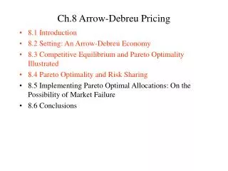
Ch.8 Arrow-Debreu Pricing • 8.1 Introduction • 8.2 Setting: An Arrow-Debreu Economy • 8.3 Competitive Equilibrium and Pareto Optimality Illustrated • 8.4 Pareto Optimality and Risk Sharing • 8.5 Implementing Pareto Optimal Allocations: On the Possibility of Market Failure • 8.6 Conclusions
8.2 Setting: An Arrow-Debreu Economy • General equilibrium • Supply = Demand • With production (if desired) • Static but Multi-period • No restrictions on preferences • The most general of the theories we shall consider
8.2 Setting: An Arrow-Debreu Economy 1. Two dates: 0, 1. This set-up, however, is fully generalizable to multiple periods. 2. N possible states of nature at date 1, which we index by q = 1,2, ...,N with probabilitiespq. 3. One perishable (non storable) consumption good; 4. K agents, indexed k = 1,...,K, with preferences: 5. In addition, agent k's endowment is described by the vector { }. Possibly:
Traded Securities: • Exclusively Arrow-Debreu securities (contingent claims): Security q priced qq promises delivery of one unit of commodity tomorrow if state q is realized and nothing otherwise • How to secure one unit of consumption to morrow?
(P) Equilibrium is a set of prices (q1, …, qN) such that 1. at those prices solve problem (P), for all k, and 2. , for every q.
8.3 Competitive Equilibrium and Pareto Optimality Illustrated
Agent 1: Agent 2: Agent 1: Agent 2: Note: q1, q2 solve « key finance problem »!
(8.3) Checking Pareto Optimality
(8.2) Box 8-1 Interior vs. Corner Solutions
If one security (q1) only (incomplete markets): • Post-trade utilities: • Agent 1: 5.51 instead of 5.62 • Agent 2: 4.03 instead of 4.09
Post-trade allocation is Pareto Optimal • After trade, EU in period 1 is approx. 1.1 for both agents.
Post-trade allocation is PO • Features perfect risk sharing or full mutual insurance (no • aggregate risk)
(8.3) Pareto optimality and risk sharing 1. If one of the two agents is fully insured, the other must be as well. 2. More generally, if the MRS are to differ from 1, given that they must be equal between them, the low consumption - high MU state must be the same for both agents and similarly for the high consumption - low MU state
3. If there is aggregate risk, however, the above reasoning also implies that, at a Pareto optimum, it is shared “proportionately” among agents with same risk tolerance. 4. Finally, if agents are differentially risk averse, in a Pareto optimal allocation the less risk averse will typically provide some insurance services to the more risk averse. 5. More generally, optimal risk sharing dictates that the agent most tolerant of risk bears a disproportionate share of it.
(i)' : - qQ + ; 8.5 Implementing Pareto Optimal Allocations: On the Possibility of Market Failure (i) Agent 1 solves : max (4 - qQ ) + [1/2 ln(1 + ) + 1/2 ln(5)] qQ 4 (ii) Agent 2 solves : max (4 -qQ ) + [1/2 ln(5 + ) + 1/2 ln(1)] qQ 4 (ii)' : - qQ + = ;
8.6 Arrow-Debreu pricing: concluding remarks • The « father » of all asset pricing relationships • A reference • Conceptual import • Hard to identify pure state of nature • Static
