Download
1 / 26
340 likes | 1.11k Vues
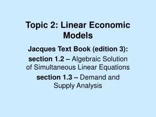
Topic 2: Linear Economic Models. Jacques Text Book (edition 3): section 1.2 – Algebraic Solution of Simultaneous Linear Equations section 1.3 – Demand and Supply Analysis. Content. Simultaneous Equations Market Equilibrium Market Equilibrium + Excise Tax Market Equilibrium + Income.

E N D
Topic 2: Linear Economic Models Jacques Text Book (edition 3): section 1.2 – Algebraic Solution of Simultaneous Linear Equations section 1.3 – Demand and Supply Analysis
Content • Simultaneous Equations • Market Equilibrium • Market Equilibrium + Excise Tax • Market Equilibrium + Income
Solving Simultaneous Equations Example • 4x + 3y = 11 (eq.1) • 2x + y = 5 (eq.2) Express both equations in terms of the same value of x (or y) • 4x = 11 - 3y (eq.1’) • 4x = 10 - 2y (eq.2’) Hence • 11 - 3y = 10 - 2y Collect terms • 11 – 10 = -2y + 3y • y = 1 Compute x • 4x = 10 - 2y • 4x = 10 – 2 = 8 • x = 2
Note that if the two functions do not intersect, then cannot solve equations simultaneously….. • x – 2y = 1 (eq.1) • 2x – 4y = -3 (eq.2) Step 1 • 2x = 2 + 4y (eq.1*) • 2x = -3 + 4y (eq.2*) Step 2 • 2 + 4y = -3 + 4y BUT => 2+3 = 0………… • No Solution to the System of Equations
Solving Linear Economic Models • Quantity Supplied: amount of a good that sellers are willing and able to sell • Supply curve: upward sloping line relating price to quantity supplied • Quantity Demanded: amount of a good that buyers are willing and able to buy • Demand curve: downward sloping line relating price to quantity demanded • Market Equilibrium: quantity demand = quantity supply
Finding the equilibrium price and quantity levels….. • In general, Demand: QD = a + bP (with b<0) Supply: QS = c + dP (with d>0) • Set QD = QS and solve simultaneously for Pe = (a - c)/(d - b) • Knowing Pe, find Qe given the demand/supply functions Qe = (ad - bc)/(d - b)
Example 1 Demand QD = 50 – P (i) Supply QS = – 10 + 2P (ii) Set QD = QS find market equilibrium P and Q • 50 – P = – 10 + 2P • 3P = 60 • P = 20 Knowing P, find Q • Q = 50 – P • = 50 – 20 = 30 Check the solution • i) 30 = 50 – 20 and (ii) 30 = – 10 + 40 In both equations if P=20 then Q=30
Example 2 Demand QD = 84 – 3P (i) Supply QS = – 60 + 6P (ii) Set QD = QS to find market equilibrium • 84 – 3P = – 60 + 6P • 144 = 9P • P = 16 Knowing P, find Q • Q = –60 + 6P • = – 60 + 96 = 36 Check the solution • 36 = 84 – (3*16) and • 36= –60 + (6*16) In both equations if P=16 then Q=36
Market Equilibrium + Excise Tax • Impose a tax t on suppliers per unit sold…… • Shifts the supply curve to the left • QD = a – bP • QS = d + eP with no tax • QS = d + e(P – t) with tax t on suppliers So from example 1…. • QD = 50 – P, • QS = – 10 + 2P becomes • QS = – 10 + 2(P-t) = – 10 + 2P – 2t cont…..
Continued….. Write Equilibrium P and Q as functions of t • Set QD = QS • 50 – P = – 10 + 2P – 2t • 60 = 3P - 2t • 3P = 60 + 2t • P = 20 + 2/3t Knowing P, find Q • Q = 50 – P • Q = 50 – (20+2/3t) • Q = 30 – 2/3t
Comparative Statics: effect on P and Q of t (i) As t, then P paid by consumers by 2/3t remaining tax (1/3) is paid by suppliers total tax t = 2/3t + 1/3t Consumers paySuppliers pay Price consumers pay – price suppliers receive = total tax t (ii) and Q by 2/3t , reflecting a shift to the left of the supply curve
For Example let t = 3 • QD = 50 – P • QS = – 10 + 2(P-t) = – 16 + 2P • New equilibrium Q = 28 (Q = 30 - 2/3t) • New equilibrium P = 22 ( P = 20 + 2/3t ) Supplier Price = 19 Tax Revenue = P*Q = 3*28 = 84
Another Tax Problem…. QD = 132 – 8P QS = – 6 + 4P • Find the equilibrium P and Q. • How does a per unit tax t affect outcomes? • What is the equilibrium P and Q if unit tax t = 4.5?
Solution….. (i) Market Equilibrium values of P and Q • Set QD = QS 132 – 8P = – 6 +4P 12P = 138 P = 11.5 • Knowing P, find Q Q = – 6 +4P • = – 6 + 4(11.5) = 40 • Equilibrium values: P = 11.5 and Q= 40
(ii) The Comparative Statics of adding a tax…… QD = 132 – 8P QS = – 6 + 4(P – t) = – 6 + 4P – 4t Set QD = QS 132 – 8P = – 6 +4P – 4t 12P = 138 + 4t P = 11.5 +1/3 t = 13 if t = 4.5 Imposing t => consumer P by 1/3t, supplier pays 2/3t Knowing P, find Q Q = 132 –8(13) = 28
(iii) If per unit t = 4.5 Tax = 0 Consumer Price = 11.5 Supplier Price = 11.5 Tax = 4.5 Consumer Price = 13 Supplier Price = 8.5 Tax Revenue = P*Q = 4.5*28 =126
Market Equilibrium and Income • Let QD = a + bP + cY Example: the following facts were observed for a good, • Demand = 110 when P = 50 and Y = 20 • When Y increased to 30, at P = 50 the demand = 115 • When P increased to 60, at Y = 30 the demand = 95
(i) Find the Linear Demand Function QD? Rewriting the facts into equations: • 110 = a + 50b + 20c eq.1 • 115 = a + 50b + 30c eq.2 • 95 = a + 60b + 30c eq.3 To find the demand function QD = a + bP + cY we need to solve these three equations simultaneously for a, b, and c
Rewriting 1 and 2 • a = 110 - 50b - 20c (eq.1*) • a = 115 - 50b - 30c (eq.2*) • => • 110 – 50b – 20c = 115 – 50b – 30c • 10c = 5 • c = ½ Rewriting 1 & 3 given c = ½ • 110 = a + 50b + 10 (eq.1*) • 95 = a + 60b + 15 (eq.3*) • a = 100 – 50b (eq.1*) • a = 80 – 60b (eq.3*) • 100 – 50b = 80 – 60b • 10b = -20 • b = -2
Given b= -2 and c = ½ , solve for a • a = 110 – 50b – 20c eq.1’ • a = 110 + 100 – 10 = 200 • QD = 200 -2P + ½Y
Now, let QS = 3P – 100 Describe fully the comparative static’s of the model using QD and QS equations? Set QD = QS for equilibrium values of P and Q • 200 -2P + ½Y = 3P – 100 • 5P = 300 + ½Y • P = 60 + 1/10Y Knowing P, find Q • Q = 3(60 + 1/10Y) -100 • = 80 + 3/10Y
What is equilibrium P and Q when Y = 20 • P = 60 + 1/10Y • P = 60 + 1/10 (20) = 62 i.e P by 1/10 of 20 = 2 • Q = 80 + 3/10Y • Q = 80 + 3/10 (20) = 86 i.e Q by 3/10 of 20 = 6
Qd = 200 – 2P + ½ Y Qs = 3P – 100 • Finding Intercepts: S(Q,P): (-100, 0) and (0, 331/3 ) Y=0: D1(Q,P): (200, 0) and (0, 100) Y=20: D2(Q,P): (210, 0) and (0, 105)
Questions CoveredTopic 2: Linear Economic Models • Algebraic Solution of Simultaneous Linear Equations • Solving for equilibrium values of P and Q • Impact of tax on equilibrium values of P and Q • Impact of Income on Demand Functions and on equilibrium values of P and Q