Download
1 / 39
390 likes | 451 Vues
Discover how significance tests determine the confidence in the existence of differences between samples in predictive modeling using paired t-tests, Student's t-distribution, and more. Learn about assessing probabilities, loss functions, and counting the costs in classification.

E N D
Significance tests • Significance tests tell us how confident we can be that there really is a difference • Null hypothesis: there is no “real” difference • Alternative hypothesis: there is a difference • A significance test measures how much evidence there is in favor of rejecting the null hypothesis • Let’s say we are using 10 times 10-fold CV • Then we want to know whether the two means of the 10 CV estimates are significantly different University of Waikato
The paired t-test • Student’s t-test tells us whether the means of two samples are significantly different • The individual samples are taken from the set of all possible cross-validation estimates • We can use a paired t-test because the individual samples are paired • The same CV is applied twice • Let x1, x2, …, xkand y1, y2, …, ykbe the 2k samples for a k-fold CV University of Waikato
The distribution of the means • Let mx and my be the means of the respective samples • If there are enough samples, the mean of a set of independent samples is normally distributed • The estimated variances of the means are x2/k and y2/k • If xand yare the true means then are approximately normally distributed with 0 mean and unit variance University of Waikato
Student’s distribution • With small samples (k<100) the mean follows Student’s distribution with k-1 degrees of freedom • Confidence limits for 9 degrees of freedom (left), compared to limits for normal distribution (right): University of Waikato
The distribution of the differences • Let md=mx-my • The difference of the means (md) also has a Student’s distribution with k-1 degrees of freedom • Let d2 be the variance of the difference • The standardized version of md is called t-statistic: • We use t to perform the t-test University of Waikato
Performing the test • Fix a significance level • If a difference is significant at the % level there is a (100-)% chance that there really is a difference • Divide the significance level by two because the test is two-tailed • I.e. the true difference can be positive or negative • Look up the value for z that corresponds to /2 • If t-z or tz then the difference is significant • I.e. the null hypothesis can be rejected University of Waikato
Unpaired observations • If the CV estimates are from different randomizations, they are no longer paired • Maybe we even used k-fold CV for one scheme, and j-fold CV for the other one • Then we have to use an unpaired t-test with min(k,j)-1 degrees of freedom • The t-statistic becomes: University of Waikato
A note on interpreting the result • All our cross-validation estimates are based on the same dataset • Hence the test only tells us whether a completek-fold CV for this dataset would show a difference • Complete k-fold CV generates all possible partitions of the data into k folds and averages the results • Ideally, we want a different dataset sample for each of the k-fold CV estimates used in the test to judge performance across different training sets University of Waikato
Predicting probabilities • Performance measure so far: success rate • Also called 0-1 loss function: • Most classifiers produces class probabilities • Depending on the application, we might want to check the accuracy of the probability estimates • 0-1 loss is not the right thing to use in those cases • Example: (Pr(Play = Yes), Pr(Play=No)) • Prefer (1, 0) over (50%, 50%). • How to express this? University of Waikato
The quadratic loss function • p1,…, pkare probability estimates for an instance • Let c be the index of the instance’s actual class • Actual: a1,…, ak=0, except for ac, which is 1 • The quadratic loss is: • Justification: University of Waikato
Informational loss function • The informational loss function is –log(pc), where c is the index of the instance’s actual class • Number of bits required to communicate the actual class • Let p1*,…, pk*be the true class probabilities • Then the expected value for the loss function is: • Justification: minimized for pj= pj* • Difficulty: zero-frequency problem University of Waikato
Discussion • Which loss function should we choose? • The quadratic loss functions takes into account all the class probability estimates for an instance • The informational loss focuses only on the probability estimate for the actual class • The quadratic loss is bounded by • It can never exceed 2 • The informational loss can be infinite • Informational loss is related to MDL principle University of Waikato
Counting the costs • In practice, different types of classification errors often incur different costs • Examples: • Predicting when cows are in heat (“in estrus”) • “Not in estrus” correct 97% of the time • Loan decisions • Oil-slick detection • Fault diagnosis • Promotional mailing University of Waikato
Taking costs into account • The confusion matrix: • There many other types of costs! • E.g.: cost of collecting training data University of Waikato
Lift charts • In practice, costs are rarely known • Decisions are usually made by comparing possible scenarios • Example: promotional mailout • Situation 1: classifier predicts that 0.1% of all households will respond • Situation 2: classifier predicts that 0.4% of the 10000 most promising households will respond • A lift chart allows for a visual comparison University of Waikato
Generating a lift chart • Instances are sorted according to their predicted probability of being a true positive: • In lift chart, x axis is sample size and y axis is number of true positives University of Waikato
A hypothetical lift chart University of Waikato
ROC curves • ROC curves are similar to lift charts • “ROC” stands for “receiver operating characteristic” • Used in signal detection to show tradeoff between hit rate and false alarm rate over noisy channel • Differences to lift chart: • y axis shows percentage of true positives in sample (rather than absolute number) • x axis shows percentage of false positives in sample (rather than sample size) University of Waikato
A sample ROC curve University of Waikato
Cross-validation and ROC curves • Simple method of getting a ROC curve using cross-validation: • Collect probabilities for instances in test folds • Sort instances according to probabilities • This method is implemented in WEKA • However, this is just one possibility • The method described in the book generates an ROC curve for each fold and averages them University of Waikato
ROC curves for two schemes University of Waikato
The convex hull • Given two learning schemes we can achieve any point on the convex hull! • TP and FP rates for scheme 1: t1 and f1 • TP and FP rates for scheme 2: t2 and f2 • If scheme 1 is used to predict 100q% of the cases and scheme 2 for the rest, then we get: • TP rate for combined scheme: q t1+(1-q) t2 • FP rate for combined scheme: q f2+(1-q) f2 University of Waikato
Cost-sensitive learning • Most learning schemes do not perform cost-sensitive learning • They generate the same classifier no matter what costs are assigned to the different classes • Example: standard decision tree learner • Simple methods for cost-sensitive learning: • Resampling of instances according to costs • Weighting of instances according to costs • Some schemes are inherently cost-sensitive, e.g. naïve Bayes University of Waikato
Measures in information retrieval • Percentage of retrieved documents that are relevant: precision=TP/TP+FP • Percentage of relevant documents that are returned: recall =TP/TP+FN • Precision/recall curves have hyperbolic shape • Summary measures: average precision at 20%, 50% and 80% recall (three-point average recall) • F-measure=(2recallprecision)/(recall+precision) University of Waikato
Summary of measures University of Waikato
Evaluating numeric prediction • Same strategies: independent test set, cross-validation, significance tests, etc. • Difference: error measures • Actual target values: a1, a2,…,an • Predicted target values: p1, p2,…,pn • Most popular measure: mean-squared error • Easy to manipulate mathematically University of Waikato
Other measures • The root mean-squared error: • The mean absolute error is less sensitive to outliers than the mean-squared error: • Sometimes relative error values are more appropriate (e.g. 10% for an error of 50 when predicting 500) University of Waikato
Improvement on the mean • Often we want to know how much the scheme improves on simply predicting the average • The relative squared error is ( ): • The relative absolute error is: University of Waikato
The correlation coefficient • Measures the statistical correlation between the predicted values and the actual values • Scale independent, between –1 and +1 • Good performance leads to large values! University of Waikato
Which measure? • Best to look at all of them • Often it doesn’t matter • Example: University of Waikato
The MDL principle • MDL stands for minimum description length • The description length is defined as: space required to describe a theory + space required to describe the theory’s mistakes • In our case the theory is the classifier and the mistakes are the errors on the training data • Aim: we want a classifier with minimal DL • MDL principle is a model selection criterion University of Waikato
Model selection criteria • Model selection criteria attempt to find a good compromise between: • The complexity of a model • Its prediction accuracy on the training data • Reasoning: a good model is a simple model that achieves high accuracy on the given data • Also known as Occam’s Razor: the best theory is the smallest one that describes all the facts University of Waikato
Elegance vs. errors • Theory 1: very simple, elegant theory that explains the data almost perfectly • Theory 2: significantly more complex theory that reproduces the data without mistakes • Theory 1 is probably preferable • Classical example: Kepler’s three laws on planetary motion • Less accurate than Copernicus’s latest refinement of the Ptolemaic theory of epicycles University of Waikato
MDL and compression • The MDL principle is closely related to data compression: • It postulates that the best theory is the one that compresses the data the most • I.e. to compress a dataset we generate a model and then store the model and its mistakes • We need to compute (a) the size of the model and (b) the space needed for encoding the errors • (b) is easy: can use the informational loss function • For (a) we need a method to encode the model University of Waikato
DL and Bayes’s theorem • L[T]=“length” of the theory • L[E|T]=training set encoded wrt. the theory • Description length= L[T] + L[E|T] • Bayes’s theorem gives us the a posteriori probability of a theory given the data: • Equivalent to: constant University of Waikato
MDL and MAP • MAP stands for maximum a posteriori probability • Finding the MAP theory corresponds to finding the MDL theory • Difficult bit in applying the MAP principle: determining the prior probability Pr[T] of the theory • Corresponds to difficult part in applying the MDL principle: coding scheme for the theory • I.e. if we know a priori that a particular theory is more likely we need less bits to encode it University of Waikato
Discussion of the MDL principle • Advantage: makes full use of the training data when selecting a model • Disadvantage 1: appropriate coding scheme/prior probabilities for theories are crucial • Disadvantage 2: no guarantee that the MDL theory is the one which minimizes the expected error • Note: Occam’s Razor is an axiom! • Epicurus’s principle of multiple explanations: keep all theories that are consistent with the data University of Waikato
Bayesian model averaging • Reflects Epicurus’s principle: all theories are used for prediction weighted according to P[T|E] • Let I be a new instance whose class we want to predict • Let C be the random variable denoting the class • Then BMA gives us the probability of C given I, the training data E, and the possible theories Tj: University of Waikato
MDL and clustering • DL of theory: DL needed for encoding the clusters (e.g. cluster centers) • DL of data given theory: need to encode cluster membership and position relative to cluster (e.g. distance to cluster center) • Works if coding scheme needs less code space for small numbers than for large ones • With nominal attributes, we need to communicate probability distributions for each cluster University of Waikato