
Programming Paradigms and Algorithms
E N D
Presentation Transcript
Programming Paradigms and Algorithms W+A 3.1, 3.2, p. 178, 6.3.2, 10.4.1 H. Casanova, A. Legrand, Z. Zaogordnov, and F. Berman, "Heuristics for Scheduling Parameter Sweep Applications in Grid Environments", Proceedings of the 2000 Heterogeneous Computing Workshop (http:apples.ucsd.edu) CSE 160/Berman
Parallel programs • A parallel program is a collection of tasks which can communicate and cooperate to solve large problems. • Over the last 2 decades, some basic program structures have proven successful on a variety of parallel architectures • The next few lectures will focus on parallel program structures and programming issues. CSE 160/Berman
Common Parallel Programming Paradigms • Embarrassingly parallel programs • Workqueue • Master/Slave programs • Monte Carlo methods • Regular, Iterative (Stencil) Computations • Pipelined Computations • Synchronous Computations CSE 160/Berman
Embarrassingly Parallel Computations • An embarrassingly parallel computation is one that can be divided into completely independent parts that can be executed simultaneously. • (Nearly) embarrassingly parallel computations are those that require results to be distributed, collected and/or combined in some minimal way. • In practice, nearly embarrassingly parallel and embarrassingly parallel computations both called embarrassingly parallel • Embarrassingly parallel computations have potential to achieve maximal speedup on parallel platforms CSE 160/Berman
Example: the Mandelbrot Computation • Mandelbrot is an image computing and display computation. • Pixels of an image (the “mandelbrot set”) are stored in a 2D array. • Each pixel is computed by iterating the complex function where c is the complex number (a+bi) giving the position of the pixel in the complex plane CSE 160/Berman
Mandelbrot • Computation of a single pixel: • Subscript k denotes kth interation • Initial value of z is 0, value of c is free parameter • Iterations are continued until the magnitude of z is greater than 2 (which indicates that eventually z will become infinite) or the number of iterations reaches a given threshold. • The magnitude of z is given by CSE 160/Berman
Sample Mandelbrot Visualization • Black points do not go to infinity • Colors represent “lemniscates” which are basically sets of points which converge at the same rate • http://library.thinkquest.org/3288/myomand.html lets you color your own mandelbrot set CSE 160/Berman
Mandelbrot Programming Issues • Mandelbrot can be structured as a data parallel computation so the same computation is performed on all pixels, except with different complex numbers c. • The difference in input parameters result in different number of iterations (execution times) for the computation of different pixels. • Mandelbrot is embarrassingly parallel – computation of any two pixels is completely independent. • Computation is generally visualized in terms of display where pixel color corresponds to the number of iterations required to compute the pixel • Coordinate system of Mandelbrot set is scaled to match the coordinate system of the display area CSE 160/Berman
Static Mapping to Achieve Performance • Pixels generally organized into blocks and the blocks are computed on processors • Mapping of blocks to processors can greatly affect application performance • Want to load-balance the work of computing the values of the pixels across all processors. CSE 160/Berman
Static Mapping to Achieve Performance • Good load-balancing strategy for Mandelbrot is to randomize distribution of pixels Block decomposition can unbalance load by clustering long-running pixel computations Randomized decomposition can balance load by distributing long-running pixel computations CSE 160/Berman
Processorsobtain block(s) from front of queue Processors Blocks Processorsperform work and get more block(s) Dynamic Mapping: Using Workqueue to Achieve Performance • Approach: • Initially assign some blocks to processors • When processors complete assigned blocks, join queue to wait for assignment of more blocks • When all blocks have been assigned, application concludes CSE 160/Berman
Workqueue Programming Issues • How much work should be assigned initially to processors? • How many blocks should be assigned to a given processor? • Should this always be the same for each processor? for all processors? • Should the blocks be ordered in the workqueue in some way? • Performance of workqueue optimized if • Computation of each processor amortizes the work of obtaining the blocks CSE 160/Berman
Master/Slave Computations • Workqueue can be implemented as a master/slave computation • Master directs the allocation of work to slaves • Slaves perform work • Typical M/S Interaction • Slave While there is more work to be done Request work from Master Perform Work (Provide results to Master) • Master While there is more work to be done (Receive results and process) Provide work to requesting slave CSE 160/Berman
Flavors of M/S and Programming Issues • “Flavors” of M/S • In some variations of M/S, master can also be a slave • Typically slaves do not communicate • Slave may return “results” to master or may just request more work • Programming Issues • M/S most efficient if granularity of tasks assigned to slaves amortizes communication between M and S • Speed of slave or execution time of task may warrant non-uniform assignment of tasks to slaves • Procedure for determining task assignment should be efficient CSE 160/Berman
More Programming Issues • Master/Slave and Workqueue may also be used with “work-stealing” approach where slaves/processes communicate with one another to redistribute the work during execution • Processors A and B perform computation • If B finishes before A, B can ask A for work A B CSE 160/Berman
Monte Carlo Methods • Monte Carlo methods based on the use of random selections in calculations which lead to the solution of numerical and physical problems. • Term refers to similarity of statistical simulation to games of chance • Monte Carlo simulation consists of multiple calculations, each of which utilizes a randomized parameter CSE 160/Berman
1 Monte Carlo Example: Calculation of P • Consider a circle of unit radius inside a square box of side 2 • The ratio of the area of the circleto the area of thesquare is CSE 160/Berman
Monte Carlo Calculation of P • Monte Carlo method to approximating : • Randomly choose a sufficient number of points in the square • For each point p, determine if p is inthe circle or the square • The ratio of points inthe circle to points in the square will providean approximation of CSE 160/Berman
p y x M/S Implementation of Monte Carlo Approximation of P • Master code • While there are more points to calculate • (Receive value from slave; update circlesum or boxsum) • Generate a (pseudo-)random value p=(x,y) in the bounding box • Send p to slave • Slave code • While there are more points to calculate • Receive p from master • Determine if p is in the circle or the square[ check to see if ] • Send p’s status to master; ask for more work CSE 160/Berman
MCell= General simulator for cellular microphysiology Uses Monte Carlo diffusion and chemical reaction algorithm in 3D to simulate complex biochemical interactions of molecules Molecular environment represented as 3D space in which trajectories of ligands against cell membranes tracked Researchers need huge runs to model entire cells at molecular level. 100,000s of tasks 10s of Gbytes of output data Will ultimately perform execution-time computational steering , data analysis and visualization Using Monte Carlo for a Large-Scale Simulation: MCell
Monte Carlo simulation performed on large parameter space In implementation, parameter sets stored in large shared data files Each task implements an “experiment” with a distinct data set Ultimately users will produce partial results during large-scale runs and use them to “steer” the simulation MCell Application Architecture
MCell Programming Issues • Application is nearly embarrassingly parallel and can target either MPP or clusters • Could even target both if implementation were developed in this way • Although application is nearly embarrassingly parallel, tasks share large input files • Cost of moving files can dominate computation time by a large factor • Most efficient approach is to co-locate data and computation • Workqueue does not consider data location in allocation of tasks to processors CSE 160/Berman
storage Cluster network links User’s hostand storage Scheduling MCell • We’ll show several ways that MCell can be scheduled on a set of clusters and compare execution performance MPP
Computation Computation Contingency Scheduling Algorithm • Allocation developed by dynamically generating a Gantt chart for scheduling unassigned tasks between scheduling events • Basic skeleton • Compute the next scheduling event • Create a Gantt Chart G • For each computation and file transfer currently underway, compute an estimate of its completion time and fill in the corresponding slots in G • Select a subset T of the tasks that have not started execution • Until each host has been assigned enough work, heuristically assign tasks to hosts, filling in slots in G • Implement schedule Network links Hosts(Cluster 1) Hosts(Cluster 2) Resources 1 2 1 2 1 2 Scheduling event Time Scheduling event G
MCell Scheduling Heuristics • Many heuristics can be used in the contingency scheduling algorithm • Min-Min [task/resource that can complete the earliest is assigned first] • Max-Min [longest of task/earliest resource times assigned first] • Sufferage [task that would “suffer” most if given a poor schedule assigned first] • Extended Sufferage [minimal completion times computed for task on each cluster, sufferage heuristic applied to these] • Workqueue [randomly chosen task assigned first]
Which heuristic is best? • How sensitive are the scheduling heuristics to the location of shared input files and cost of data transmission? • Used the contingency scheduling algorithm to compare • Min-min • Max-min • Sufferage • Extended Sufferage • Workqueue • Ran the contingency scheduling algorithm on a simulator which reproduced file sizes and task run-times of real MCell runs. CSE 160/Berman
Workqueue Sufferage Max-min Min-min XSufferage MCell Simulation Results • Comparison of the performance of scheduling heuristics when it is up to 40 times more expensive to send a shared file across the network than it is to compute a task • “Extended sufferage” scheduling heuristic takes advantage of file sharing to achieve good application performance
Additional Programming Issues • We almost never know completely accurately what the runtime will be • Resources may be shared • Computation may be data dependent • Task execution time may be hard to predict • How sensitive are the scheduling heuristics to inaccurate performance information? • i.e., what if our estimate of the execution time of a task on a resource is not 100% accurate? CSE 160/Berman
MCell with a single scheduling event and task execution time predictions with between 0% error and 100% error