Solutions of Nonelectrolytes

1. Solutions of Nonelectrolytes

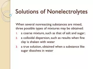
2. Introduction A true solution is defined as a mixture of two or more components that form a homogenous molecular dispersion, in other words, a one-phase system, the composition of which can vary over a wide range.

3. Types of solutions

4. Types of Solutions • The solutes (whether gases, liquids, or solids) are divided into two main classes: nonelectrolytes and electroytes. • Nonelectrolytes are substances that do not yield ions when dissolved in water and therefore do not conduct an electric current through the solution. • Examples of noneletrolytes are sucrose, glycerin, naphthalene, and urea.

5. Types of Solutions • Electrolytes are substances that form ions in solutions, conduct the electric current. • Examples of electrolytes are hydrochloric acid, sodium sulfate, ephedrine, and phenobarbital. • Electrolytes may be subdivided further into strong electroytes (hydrochloric acid, sodium sulphate) and weak electrolytes (ephedrine, phenobarbital).

6. Concentration Expressions

7. Equivalent Weights

8. Equivalent Weights

9. Example: An aqueous solution of ferrous sulfate was prepared by adding 41.5 g of FeSO4 to enough water to make 1000 ml of solution at 18°C. The density of the solution is 1.0375 and the molecular weight of FeSO4 is 151.9. Calculate: • The molarity. • The normality. • The molality. • The mole fraction and mole percent for both solute and solvent. • The percentage by weight of FeSO4. Answer: a) Molarity = moles of FeSO4/Liters of solution = (41.5/151.9)/ 1 L = 0.2732 M. b) Normality = (41.5/ 75.95)/ 1L= 0.5464 N c) Molality = moles of FeSO4/ kg of solvent = 0.2732/ 0.996= 0.2743 m Equivalent weight= 151.9/2= 75.95 g/Eq Grams of solution = volume * density = 1000 * 1.0375= 1037.5 g Grams of solvent = 1037.5- 41.5= 996 g

10. Example…….cont.: d) Mole fraction and mole percent: Moles of water = n1= 996/18.02= 55.27 moles. Moles of FeSO4 = n2 = 0.2732 moles. Mole fraction of water = X1 = 55.27/ (55.27 + 0.2732) = 0.9951 Mole percent of water = 0.9951 * 100%= 99.51%. Mole fraction of FeSO4= X2= 0.2732/ (55.27 + 0.2732) = 0.0049 Mole percent of FeSO4= 0.49% e) Percentage by weight of FeSO4= (g of FeSO4/ g of solution) *100 = (41.5/ 1037.5) *100 = 4 %

11. Solution properties • Solution properties may be classified as extensive properties , depending on the quantity of the matter in the system (e.g. mass and volume) and intensive properties, which are independent of the amount of substances in the system (e.g. temperature, pressure, density, surface tension, and viscosity of pure liquids). • Solution properties can also be classified as additive, constitutive and colligative. • Additive properties are derived from the sum of the properties of the individual atoms or functional groups within the molecule e.g. mass • Constitutive properties are dependent on the structural arrangement of the atoms within the molecule e.g. optical rotation. • Colligative properties will be discussed soon later.

12. Ideal solutions • Ideal solutions are formed by mixing substances with similar properties. • Ideality in solution means complete uniformity of attractive forces (i.e. cohesive forces between A molecules are similar to cohesive forces between B molecules; both of which are similar to the adhesive forces between A and B molecules). • Ideal solution is the solution in which there is no change in the properties of the components, other than dilution, when they are mixed to form the solution. • In ideal solution, no heat is evolved or absorbed during the mixing process, and the final volume of the solution represents an additive property of the individual constituents. No shrinkage or expansion occurs when substances are mixed together (e.g. a solution of methanol and ethanol).

13. Escaping Tendency • When two bodies are in contact with each other and one is heated to a higher temperature than the other, heat will flow from the hotter to the colder body until the bodies are in thermal equilibrium. This process is termed the escaping tendency. • The hotter body has a greater escaping tendency until the temperature of both bodies is the same. • Temperature is a quantitative measure of escaping tendency of heat.

14. Escaping Tendency • Free energy is a quantitative measure of escaping tendencies of substances undergoing physical and chemical transformations – for a pure substance, it is the molar free energy, for a solution, it is the partial molar free energy. • Free energy of a mole of ice is greater than that of a liquid water at 1 atm above 0ºC. • Above 0ºC, The escaping tendency of ice is greater than that of liquid water, so ice is converted to water. • At 0ºC, the escaping tendencies of ice and water are the same, G = 0.

15. Raoult’s Law • Raoult’s Law applies for solvents while Henry’s law applies for solutes. • Activity, “effective concentration”, is a term used to describe departure of the behavior of a solution from ideality. In an ideal solution or in a real solution at infinite dilution there is no interactions between components and the activity equals the concentration (activity = concentration).

16. Raoult’s Law • The activity, in general, is less than the actual or stoichiometric concentration of the solute as interactions occur between the components which reduce the effective concentration of the solute. • Non-ideality in real solutions at high concentrations causes a divergence between the values of activity and concentration. The ratio of the activity to the concentration is called the activity coefficient, .

17. Raoult’s Law • Depending on the units used to express the concentration we can have either a molal activity coefficient, m, a molar activity coefficient, c, or if mole fractions are used, a rational activity coefficient, x. where m is the molality, c is the molar concentration, x is the mole fraction.

18. Raoult’s Law • The activity coefficient is a proportionality constant relating activity to concentration. • The activity coefficient usually decreases and assumes different values as the concentration increases. • Differences among the three activity coefficients may be disregarded in dilute solutions in which c  m 0.01. • The concept of activity and activity coefficient may be applied to nonelectrolytes, weak as well as strong electrolytes.

19. Raoult’s Law- Ideal solutions • The vapor pressure of a solution is a quantitative expression of escaping tendency. • Raoult’s law: In an ideal solution, the partial vapor pressure of each volatile constituent is equal to the vapor pressure of the pure constituent multiplied by its mole fraction in the solution. Pt= P1ºX1 + P2ºX2 where P1ºX1 and P2ºX2are the partial vapor pressures of the pure components when the mole fractions are X1 and X2. P1º and P2º are the vapor pressure of the pure components.

20. Raoult’s Law- Ideal solutions • So in ideal solutions, when liquid A is mixed with liquid B, the vapor pressure of A is reduced by dilution with B in a manner depending on the mole fractions of A and B present in the final solution. This will diminish the escaping tendency of each constituent , leading to a reduction in the rate of escape of the molecules of A and B from the surface of the liquid.

21. The activities and activity coefficients of solvents on the assumption of ideal-gas behavior of the vapor

22. The vapor pressures of the components and the total vapor pressures for the nearly ideal solution benzene-toluene at 20ºC

23. Raoult’s Law- Ideal solutions Total vapor pressure PB°= 268 PA°= 236 PB°XB PA°XA Vapor pressure (mm Hg) Ethylen Chloride XA= 1 Mole fraction of Ethylen Chloride Benzene XB= 1

24. Real (nonideal) solutions • Many examples of solution pairs are known in which the “cohesive” attraction of A for A exceeds the “adhesive” attraction existing between A and B. Similarly, the attractive forces between A and B may be greater than those between A and A or B and B. This may occur even though the liquids are miscible in all proportions. Such mixtures are real or nonideal.

25. Real (nonideal) solutions Negative deviation: When “adhesive” attractions between molecules of different species exceed the “cohesive” attractions between like molecules, the vapor pressure of the solution is less than expected from Raoult’s ideal solution law, and negative deviation occurs. Pt P1ºX1 + P2 ºX2  a1X1 , a2 X2  Pt = P1ºa1 +P2ºa2 Example: chlorofrom and acetone – due to formation of hydrogen bonds thus reducing the escaping tendency of each other. Cl3C-H……O=C(CH3)2

26. The activities and activity coefficients of solvents showing negative deviation from Raoult’s law Note: with dilution, a→c, →1

27. Vapor pressure diagram for the system chloroform-acetone at 35C

28. Real (nonideal) solutions Positive deviation: When interaction between A and B molecules is less than that of the pure constituents, the presence of B molecules reduce the interaction of A molecules, and A molecules reduce B-B interaction  greater escaping tendency of A and B molecules  partial vapor pressure of the constituents is greater than that expected from Raoult’s law. Pt P1ºX1 + P2ºX2  a1 X1 ,a2 X2  Pt= P1ºa1 +P2ºa2 Examples: benzene and ethyl alcohol, carbon disulfide and acetone, chloroform and ethyl alcohol, carbon tetrachloride and methyl alcohol

29. The activities and activity coefficients of solvents showing positive deviation from Raoult’s law Note: dilution of the dimer structure in alcohol → increases the vapor pressure of the alcohol

30. Vapor pressure diagram for the system carbon tetrachloride (CCl4) – methyl alcohol (CH3OH) at 35C

31. Real (nonideal) solutions • In real solutions, Raoult’s law does NOT apply over the entire concentration range. It can only be applicable for a substance with high concentration (i.e. solvents in real solutions). For the previous figures (slides 18 and 20), you can observe that the actual vapor pressure curve of subtances approach the ideal curve defined by Raoult’s law at high concentrations (being solvent).

32. Raoult’s Law • If you have the fourth edition of the book, solve problems 5-9 and 5-10 page 122, and problems 6-27 and 6-28 page 142. • If you have the fifth edition of the book, solve problems 5-9 and 510 page 693, and problems 6-27 page 697 and 6-28 page 698.

33. Colligative properties • Colligative properties depend mainly on the number of particles in a solution. • The value of the colligative properties are approximately the same for equal concentrations of different nonelectrolytes in solution regardless of the species or chemical nature of the constituents. • The colligative properties of solutions are: osmotic pressure, vapor pressure lowering, freezing point depression, and boiling point elevation. • In considering the colligative properties of solid-in-liquid solutions, it is assumed that the solute is nonvolatile and that the pressure of the vapor above the solution is provided entirely by the solvent.

34. Colligative properties • The colligative properties of solutions of nonelectrolytes are fairly regular. A 0.1 M solution of a nonelectroyte produces approximately the same colligative properties as any other nonelectrolyte solution of equal concentrations. • Solutions of electrolytes show apparent “anomalous” colligative properties, that is, they produce a considerably greater freezing point depression and boiling point elevation than do nonelectrolytes of the same concentration.

35. Lowering of Vapor Pressure, P • When a nonvolatile solute is combined with a volatile solvent, the vapor above the solution is provided solely by the solvent. The solute reduces the escaping tendency of the solvent, and, on the basis of Raoult’s law, the vapor pressure is lowered proportional to the relative number (rather than the weight concentration) of the solute molecules. • Since the solute is nonvolatile, the vapor pressure of the solvent P1 is identical to the total pressure of the solution P. • It is more convenient to express the vapor pressure of the solution in terms of the solvent.

36. Lowering of Vapor Pressure, P • X1 is the solvent mole fraction and X2 is the solute mole fraction X1 + X2 = 1 i.e. X1 = 1- X2 so P = P1º (1 – X2)  P1º – P = P1ºX2 thus Where ΔP is the lowering of the vapor pressure and ΔP/P1° is the relative vapor pressure lowering. • As ΔP/P1° depends only on the number of solute molecules, it is considered as a colligative property.

37. Lowering of Vapor Pressure, P • For dilute solutions (n2n1) so • When water is the solvent, 1000g = 1L Thus where m is the solute molatity (Why in molality, not in molarity or normality?)

38. Lowering of Vapor Pressure, P Q) Calculate the relative vapor pressure lowering at 20°C for a solution containing 171.2 g of sucrose in 1000g of water. The molecular weight of sucrose is 342.3 and the molecular weight of water is 18.02. Moles of sucrose (n2) = 171.2/342.3= 0.5 mol Moles of water (n1)= 1000/18.02= 55.5 mol ΔP/P1°= X2= 0.5/ (0.5+55.5)= 0.0089. Q) For the above question, providing that the vapor pressure of water at 20°C is 17.54 mm Hg. Calculate the vapor pressure when added 171.2 g of sucrose (0.5 mol). ΔP/P1°= (P1°- P)/ P1°= (17.54-P)/17.54=0.0089 P= 17.38 mmHg

39. Elevation of the Boiling Point • The boiling point of a solution of a nonvolatile solute is higher than that of the pure solvent, owing to the fact that the solute lowers the vapor pressure of the solvent. Figure – Boiling point elevation of the solvent due to addition of a solute (not to scale) The elevation of the boiling point can be written as T – Tº = Tb

40. Elevation of the Boiling Point • An exact equation to calculate Tb (boiling point elevation) where Hv is the latent heat of vaporization of the solvent, Tb is the boiling point of the solvent, R is the gas constant, X2 is the mole fraction of the solute • A less exact equation (more commonly used) is where M1 is the molecular weight of the solvent, m is the molal concentration of the solute (mol.kg-1), Kb is the molal elevation constant or the ebullioscopic constant (deg.kg.mol-1)

41. Elevation of the Boiling Point • Kb (ebullioscopic constant) has a characteristic value for each solvent; Kb for water is 0.51 deg.kg/mole. • Kb may be considered as the boiling point elevation for an ideal 1m solution. • Stated another way, Kb is the ratio of the boiling point elevation to the molal concentration in an extremely dilute solution in which the system is approximately ideal.

42. Elevation of the Boiling Point Figure - the influence of concentration on the ebulioscopic constant.

43. Depression of Freezing Point • The normal freezing point or melting point of a pure compound is the temperature at which the solid and the liquid phases are in equilibrium under a pressure of 1atm. Equilibrium here means that the tendency for the solid to pass into the liquid is the same as the tendency for the reverse process to occur, since both the liquid and the solid have the same escaping tendency. • The T value for water saturated with air at this pressure is arbitrary assigned a temperature of 0ºC – see figure. • The triple point of air-free water, at which solid, liquid, and vapor are in equilibrium, lies at a pressure of 4.58 mmHg and a temperature of 0.0098ºC.

44. Depression of Freezing Point Figure – Depression of the freezing point of the solvent, water, by a solute ( not to scale).

45. Depression of Freezing Point • The more concentrated is the solution, the farther apart are the solvent and the solution curves and the greater is the freezing point depression (Tf). • Tf is proportional to the molal concentration of the solute and can be determined as follows: Tf = Kfm or or where Tf is the freezing point depression, Hf is molal heat of fusion, Tf is the freezing point of the solvent and Kf is the molal depression constant or the cryoscopic constant, which depends on the physical and chemical properties of the solvent, Kf for water is 1.86 deg.kg/mole.

46. Depression of Freezing Point • The freezing point depression of a solvent is a function only of the number of particles in the solution, and for this reason it is referred to as a colligative property. • The depression of the freezing point, like the boiling point elevation, is a direct result of the lowering of the vapor pressure of the solvent. • Kf may be determined experimentally by measuring Tf/m at several molal concentrations and extrapolating to zero concentration – i.e. Kf is the intercept. Electrolytes don’t follow this relationship. The equation is

47. Depression of Freezing Point Figure – The influence of concentration on the cryoscopic constant for water

48. Depression of Freezing Point • Citric acid shows abnormal behavior as seen in the previous figure – This abnormal behavior is to be expected when dealing with electrolytes. • Freezing point depression can also be calculated from the following equation: where Tf is the freezing point of the solvent, T is the freezing point of the solution, X2 is the mole fraction of the solute, R is the gas constant and Hf is the heat of fusion of the solvent.

49. Osmotic Pressure  • Escaping tendency can be measured in terms of vapor pressure or the closely related colligative property, osmotic pressure. • If a solution is confined in a membrane only permeable to the solvent molecules (semipermeable), osmosis occurs. • Osmosis is defined as the passage of the solvent into a solution through a semi-permeable membrane.

50. Osmotic Pressure  Apparatus for demonstrating osmosis.