Download
1 / 31
310 likes | 421 Vues
Example of Models for the Study of Change. David A. Kenny. Example Data. An Honors Thesis done by Allison Gillum of Skidmore College supervised by John Berman on the effects of an semester-long class on the Environment on Environmental Responsible Behaviors. Pretest-Posttest Design

E N D
Example of Models for the Study of Change David A. Kenny
Example Data An Honors Thesis done by Allison Gillum of Skidmore College supervised by John Berman on the effects of an semester-long class on the Environment on Environmental Responsible Behaviors. Pretest-Posttest Design 41 Treated and 199 Controls 2 Treated classes and 8 Control classes. No clustering effect due to class. Outcome: Environmentally Responsible Behaviors (ERB), a 12 item scale ranging for 1 to 7. For latent variable analyses, 3 parcels of 4 items were created.
Models • Models • Controlling for Baseline • Simple • Allowing for Unreliability at Time 1 • Change Score Analysis • Raykov • LCS • Kenny-Judd • Standardized Change Analysis • Types • Univariate (average of 12 items) • Latent Variable (3 parcels of 4 items)
Latent Variable Measurement Models • Unconstrained • c2(9) = 13.22, p = .153 • RMSEA = 0.044; TLI = .992 • Equal Loadings • c2(11) = 18.63, p = .068 • RMSEA = 0.054; TLI = .988 • The equal loading model has reasonable fit.
Pretest Difference • Mean for Controls: 4.79 • Mean for Treateds: 5.21 • A mean difference of 0.42 • t(238) = 3.191, p = .002 • d = 0.64, a moderate effect size • There is a difference at the pretest! • The mean difference on latent variable at time 1 is 0.45.
More on the Pretest Difference • Likely more environmentally conscious students more likely to take an environmental course. • Would you expect the difference to persist (CSA) or narrow (CfB)?
Controlling for Baseline: Univariate • A beneficial effect of the course on the outcome: 0.3049. • Z = 3.992, p < .001 • b = 0.776 (expect a narrowing of the gap) • We shall see that this is the largest estimate of the treatment effect.
CfB: Measurement Error in the Pretest Coefficient alpha of .872 for pretest Lord-Porter Correction Convert (.872 - .2112)/( 1 - .2112) = .866 Adjusted pretest score (MT is the mean for the Treated and MC is the mean for the controls): r(X1 – MT) + MT r(X1 – MC) + MC b = 0.2569, Z = 3.3308, p < .001
Williams & Hazer Method Set X1 = X1T + E1 Fix the variance of E1 to (1 - r)sY12 or (1 - .872)(0.614) = 0.079. b = 0.2543, Z = 3.233, p = .001 (with b = .897) Same estimates of b and b as Lord-Porter (standard error a bit different)!
Controlling for Baseline: Latent Variables • b = 0.3256, Z = 4.124, p < .001 • b = 0.816 (surprisingly relatively low) • Cannot directly compare estimates to the univariate analysis.
Change Score Analysis: Univariate • All 3 methods (see next 3 slides) show a beneficial effect: • 0.2105, Z = 2.619, p = .009 • Smallest effect of any analysis, • Note that the Treateds improve (0.0874), and the Controls decline (-0.1231).
Change Score Analysis: Latent Variables • All 3 methods show a beneficial effect 0.2435, Z = 2.964, p < .003 • Again, you cannot directly compare the univariate and latent variable results. • Smallest effect of any latent variable analysis.
Standardized Change Score Analysis: Univariate Analysis Residual variance decreases slightly over time (but not significantly, p = .31) • Time 1: 0.59 • Time 2: 0.52 Effect: .3078, Z = 2.775 , p = .006 Recalibrated to units of Time 2: 0.2266 , Z = 2.826 , p = .005.
Standardized Change Score Analysis: Latent Variables Residual variance decreases slightly over time (but not significantly, p = .30) • Time 1: 0.56 • Time 2: 0.52 b = 0.3653, Z = 3.116 , p = .002 Units of Time 2: b = 0.2627, Z = 3.194 , p = .001
Summary of Univariate Effects CfB: 0.3049 CfB with Reliability Correction: 0.2543 CSA: 0.2105 SCSA: 0.2266
Summary of Latent Variable Effects CfB: 0.3256 CSA: 0.2435 SCSA: 0.2627
What Estimate Would I Report? CSA Latent Variable: 0.2435 (Z = 2.964, p < .003) No reason to think that the factors that created the Time 1 difference to change. Note too the variance does not change. Others might respectfully disagree.