Download
1 / 40
400 likes | 577 Vues
OMI NO 2 observations of boreal forest fires. Nicolas Bousserez. Why studying NO 2 ?. NO x = NO+NO 2 is the main O 3 precursor with VOCs in the troposphere NO x is an harmful pollutant at urban concentrations (mostly during winter)

E N D
OMI NO2 observations of boreal forest fires Nicolas Bousserez
Why studying NO2? • NOx = NO+NO2 is the main O3 precursor with VOCs in the troposphere • NOx is an harmful pollutant at urban concentrations (mostly during winter) • NOx has a short lifetime (≈hours in summer) but can be transported over long distance through reservoir species (PAN) Regional to intercontinental transport of pollution
OMI NO2 retrieval(DOAS method) • AMF formulation : Ωv = Ωs /AMF Ωv = Vertical Column Ωs = Slant Column Spectral fitting AMF = Air Mass Factor Radiative transfert calculation Geometric correction Scattering weights (Radiative transfert model) Shape factor: normalized NO2 profile (model output)
Motivation • Boersma (2004): • Shape factor uncertainty < 15% • “Cloud algorithms implicitly correct for aerosol through their modified cloud fraction and height”. • Forest fires emit large amount of both aerosols and NOx Testing the impact of shape factor and aerosol correction over fires
ARCTAS experimentSpring/Summer 2008 • Summer phase (June, 18 - July, 13) • Boreal forest fires over center Canada • DC-8 measurements: • NOx concentrations • Aerosols optical properties
MODIS AOD OMI NO2 2008/06/18-2008/07/13 average
GEOS-Chem ARCTAS NRT Simulations • GEOS-Chem v8-01-01 • Modifications: • David Streets 2006 emissions over SE Asia & China • FLAMBE daily biomass burning emissions • GEOS-5 Metfields • Horizontal Grid: 2º lat x 2.5º lon • Vertical Grid: Reduced 47 layers
Emissions modifications • Assume that EFco = Mco/MDM (k/kg) is correct • Use model CO bias to correct for DM burned amount • Use model Black Carbon bias to correct for smoke emission • Use a lower NOx/CO emission ratio: NOx/CO = 3.10-3 (Alvarado pers. com.) Mass CO emitted Mass Dry Matter burned
Model/in situ comparison over fires Average over Canada domain from 2008/06/18 to 2008/07/13 Original simul DC-8 obs Corrected simul Pressure (hPa) NO2 (pptv) Extinction (Mm-1) Good agreement with observation using modified FLAMBE emission inventory
Model/in situ comparison over fires DC-8 GC SSA Mostly scattering aerosols
AMF Sensitivity Study • Sensitivity to Shape factor: AMF computed with GC shape profiles from a simulation with and without Canadian biomass burning emissions • Sensitivity to aerosol correction: AMF computed with and without aerosol treatment in LIDORT
Aerosol correction vs shape factor impact 2008/07/01 High forest fire event Aerosol correction factor ≈1.4 over fires Shape correction factor ≈0.4 over fires
Biomass burning aerosols effect on shape factor correction Shape correction factor without biomass burning aerosols ≈20% decrease with bb aerosols Shape correction factor with biomass burning aerosols
Interpretation w/ fires w/o fires Shape factors Fires area Hudson area Aerosol Extinction (Hudson area) Aerosol Extinction (Fires area) Scattering weights
In situ NO2 column and AOD over fires • We select data with : • CO > 20% CO backg +CO backg • HCN > 20% HCN backg +HCN backg • In situ data binned to a 1°x1° horizonal, 1hPa vertical grid • Retain only pixels with data below 700hPa • Extrapolation method: Profile scaled to a mean in situ profile
DC-8 NO2 tropospheric columns 2008/06/18 to 2008/07/13 DC-8 Aerosol Optical Depth 2008/06/18 to 2008/07/13
OMI NO2 and MODIS AOD over fires • Select OMI pixels with distance to MODIS fires pixels < 5 km • Select MODIS pixels with distance to OMI pixels < 5 km • Pixels selected the same date as DC-8 measurements
Impact of shape factor on NO2 retrieval DC-8 observations OMI KNMI (no daily resolved biomass burning emis.) OMI KNMI with GC shape factor (KNMIGC) AOD (MODIS, DC-8) Significant impact of shape factor when AOD > 0.3
Interpretation For one case where OMI KNMI/OMI KNMIGC > 1.5 Shape factor, S*w S*w KNMIGC Californian/Asian pol. Shape factor KNMIGC S*w KNMI Shape factor KNMI Scattering weights KNMI Upper tropospheric NO2 pic responsible for higher AMF using GC shape profile Long-range transport of pollution has a significant impact on shape profile
NO2 column/AOD relationship over fires robs = 0.85 Y=0.03+0.39*X rKNMI = 0.69 rKNM GC = 0.8 rKNMI = 0.66 rKNM GC = 0.77 YKNMI=0.13+0.08*X YKNMI GC=0.10+0.15*X YKNMI=0.13+0.06*X YKNMI GC=0.11+0.10*X w/o correction w/ correction Proposed aerosol correction: For AOD > 0.3 apply an aerosol correction factor of 0.7 to the NO2 tropospheric column
Conclusion and perspectives • Neglecting aerosol correction over fires can lead to an overestimation of about 30% of the NO2 column • Shape profiles not representative of fires events can lead to an underestimation of a factor 2 of the NO2 column • Missing of upper tropospheric long-range transported pollution events in the shape profile can lead to an overestimation of 50-60 % Both local and remote emission sources play an important role • Still significant sources of error: Simulations with higher grid resolution should improve the shape profile (higher concentrations in plumes, thin structures better reproduced)
Motivation • O3 plays a key role in the oxidizing capacity of the troposphere through OH production by its photolysis • O3 has a significant radiative effect • Lightning accounts for more than 28% of the tropical troposheric O3 (Sauvage et al., 2007) • Need for vertically resolved measurements to understand Tropical Atlantic O3 distribution and seasonal variability (Jourdain et al., 2007)
TES instrument • High resolution Fourier Transform Spectrometer (FTS) on Aura • Nadir IR emission • Launched 2004 July, 15 • ≈705 km sun-sync orbit Provides CO, O3 profiles
Does TES detect ozone enhancements related to lightning NOx?Measurements-based method • Pb: Ozone concentrations impacted by both lightning and biomass burning sources • CO tracer of African biomass burning sources Look for O3/CO anomalies anticorrelation
Case study: 2006/08/02 TES Ozone at 464.16 hPa Case selected from box-averaged TES CO and TES O3 time series at 464 hPa
Global chemistry modeling: GEOS-Chem model • GEOS-Chem v8.01.04 • Horizontal grid resolution: 2.5°x2° • GEOS-4 metfields • Sensitivity simulations with and without the lightning NOx emission sources.
TES O3 (box-averaged) GC O3 (box-averaged) with averaging kernel applied
Ozone sensitivity to lightning O3 w/ lightning – O3 w/o lightning
IASI/METOP • 12 km pixel x 4 @ nadir • 120 spectra along the swath (±48.3° Scan 2400 km), each 50 km along the trace • Spectral coverage: 645-2760 cm-1 • Spectral resolution = 0.5 cm-1 • Radiometric noise ~ 0.1-0.2 K MetOP IASI Nadir looking FTS IASI instrument and status Infrared Atmospheric Sounding Interferometer Thermal IR (October 2006-) Priorities: Numerical Weather Predictions Temperature and humidity profiles each kilometer in the troposphere, (1 K, 10 % accuracy) Tropospheric chemistry and climate Integrated concentrations or vertical profiles for a series of target trace gases Global coverage twice a day (Morning and evening orbits) Timeline and data rate: Oct. 19, 2006 MetOp-A launch Nov. 29, 2006 First spectra Jun. 4, 2007 L1C Operational dissemination Sep. 27, 2007 L2 (P, T, clouds) operational dissemination Mar. 1, 2008 L2 (trace gases) operational dissemination 1.3x10⁶ spectra / day D. Hurtmans, Assfts 14, Firenze From Catherine Wespes, Halifax, May 2009
GEOS-Chem HNO3 tropospheric column with IASI averaging kernel applied
Conclusion and perspectives • Combining TES O3 and CO data provide a measurement-based assessment of the lightning-NOx influence on tropical ozone • TES analysis in combination with IASI HNO3 looks promising • A GEOS-Chem adjoint analysis will allow to map the LiNOx emission regions with most impact on tropical tropospheric ozone