Efficiency %
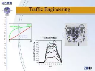
80%. Efficiency %. 41. Capacity, Erlangs. Traffic by Hour. 100%. 1. 50. 90%. 80%. 70%. 60%. 50%. 40%. 30%. 20%. 10%. 0%. Hour. Traffic Engineering. Objectives. Identify the role and functions of traffic engineering in a wireless system

Efficiency %
E N D
Presentation Transcript
80% Efficiency % 41 Capacity, Erlangs Traffic by Hour 100% 1 50 90% 80% 70% 60% 50% 40% 30% 20% 10% 0% Hour Traffic Engineering
Objectives • Identify the role and functions of traffic engineering in a wireless system • Understand the basic units and concepts of traffic engineering • Understand basic principles of system dimensioning • Develop operational familiarity with traffic tables • Understand and apply the concept of trunking efficiency to wireless systems • Examine current methods of wireless traffic forecasting and analysis
Outline • Traffic Engineering and System Dimensioning Objectives • Basics of Traffic Engineering • trunk concept • units of traffic measurement • offered traffic and call duration • blocking probability and grade of service • capacity and utilization efficiency as a function of number of trunks • Traffic Tables and Formulas • Variation of Traffic with Time • Real-System Example and Busy-hour determination • Typical Traffic Profile of Cellular System • Traffic Estimation and Cell Trunk Dimensioning • Geographic Distribution of Traffic and its estimation • for new systems, for growth cells • Exercise
$ 7 6 1 9 3 7 4 1 2 8 9 3 6 7 1 2 5 8 10 9 3 11 2 8 4 6 Traffic Engineering Objectives Traffic engineering is the intelligent art of having adequate capacity, but not spending too much to get it • Traffic engineering is applied during every stage in the development and operation of a cellular system • In Initial Design: • How many cells are needed? • What about switching resources? • What is the optimal way to backhaul? • Ongoing during Operation: • What BTS resources, and when? • When are new BTSs needed? • Anticipate resource requirements to allow budgeting and installation
BTS BTS BTS BTS BTS BTS BTS BTS BTS BTS BTS BTS BTS BTS BTS Walking a Fine Line The traffic engineer must walk a fine line between two problems: • Overdimensioning • too much cost • insufficient resources to construct • traffic revenue is too low to support costs • Underdimensioning • blocking • poor technical performance (interference) • capacity for billable revenue is low • revenue is low due to poor quality • users unhappy, cancel service
Basics of Traffic EngineeringTerminology & Concept of Trunks • Traffic engineering in telephony is focused on the voice paths users occupy. They are called by various names: • trunks • circuits • voice paths • Some other common terms are: • trunk group • a trunk group is several trunks going to the same destination, combined and addressed in switch translations as a unit , for traffic routing purposes • member • one of the trunks in a trunk group • In a CDMA system, the air interface is soft- squeezed. But there are other hard resources to be dimensioned: • Vocoders in the BSC • Channel elements in the BTS
Units of Traffic Measurement Traffic is expressed in units of Circuit Time General understanding of telephone traffic engineering began around 1910. An engineer in the Danish telephone system, Anger K. Erlang, was one of the first to develop the concepts of trunk dimensioning and publish the information for the benefit of others. In his honor, the basic unit of traffic is named the Erlang. • An Erlang of traffic is one circuit continuously used during an observation period normally one hour long -- I.e., one hour of talk. Other units have become popular among various users: • CCS (Hundred-Call-Seconds) • MOU (Minutes Of Use) • It is easy to convert between traffic units if the need arises: 1 Erlang = 60 MOU = 36 CCS
Typical CDMA System Design Blocking Probabilities PSTN Office BTS P.005 BTS P.02 MTX BSC BTS P.001 P.005 Principles of Traffic EngineeringBlocking Probability / Grade of Service • Blocking is inability to get a circuit when one is needed • Probability of Blocking is the likelihood that blocking will happen • In principle, blocking can occur anywhere in a cellular system: • not enough channel elements, the BTS is full • not enough vocoders in the BSC • not enough paths through the switching complex • not enough trunks from switch to PSTN • Blocking probability is usually expressed as a percentage : : • P.02 is 2% probability, etc. • Blocking probability sometimes is called grade Of Service • Most blocking in cellular systems • occurs at the BTS level. • P.02 is a common goal
PSTN or other Wireless user Carried Traffic MTX BSC Offered Traffic Blocked Traffic BTS BTS BTS BTS BTS BTS Offered and Carried Traffic • Offered Traffic is what users attempt to originate. • Carried Traffic is the traffic actually successfully handled by the system • Blocked traffic is the traffic that could not be handled • since blocked call attempts never materialize, blocked traffic can only be estimated based on number of blocked attempts and average duration of successful calls TO = CA x CD TO= offered traffic (any desired units) CA = total call attempts CD = average successful call duration (TO and CD must be in same units)
Ticket Counter Analogy Servers Queue User Population Traffic Engineering and Queuing Theory • Traffic Engineering is an application of a science called queuing theory • Queuing theory relates user arrival statistics, number of servers, and various queue or waiting strategies, with the probability of a user receiving service meeting specified criteria • If waiting is not allowed, and a blocked call simply goes away, Erlang-B formula applies (popular in wireless) • If unlimited waiting is allowed before service, the Erlang-C formula applies • If a wait is allowed but is limited in time, blocked calls held, Binomial & Poisson formulae apply • Fast, short transactions with no wait allowed: Engset formula applies Queues we face in Everyday Life 1) for telephone calls, 2) at the bank 3) at the gas station 4) at the airline counter
Number of Trunks vs. Utilization Efficiency Erlang-B P.02 GOS Trks Erl Eff% 1 0.02 2% 2 0.22 11% 80% Efficiency % 41 Capacity, Erlangs 1 50 • Imagine a BTS with just one voice channel. It can carry an erlang. But at a P.02 Grade of Service, how much traffic could it carry? • The trunk can only be used 2% of the time, otherwise the blocking will • be worse than 2%. • 98% availability forces 98% idleness. It can only carry .02 Erlangs. Efficiency 2%! • Adding just one trunk relieves things greatly. Now we can use • trunk 1 heavily, with trunk 2 handling the overflow. • Efficiency rises to 11% The Principle of Trunking Efficiency • For a given grade of service, trunk utilization efficiency increases as the number of trunks in the pool grows larger. • For trunk groups of several hundred, utilization approaches 100%. # Trunks
Capacity and Trunk Utilization Erlang-B for P.02 Grade of Service 45 90 40 80 35 70 30 60 25 50 20 40 15 30 10 20 5 10 0 0 0 10 20 30 40 50 Trunks Number of Trunks,Capacity, and Utilization Efficiency • The graph at left shows the capacity in erlangs for a given number of trunks, as well as the utilization efficiency • For accurate work, tables of traffic data are available • Capacity, Erlangs • Blocking Probability (GOS) • Number of Trunks • Notice how capacity and utilization behave for the numbers of trunks in typical cell sites Utilization Efficiency Percent Capacity, Erlangs
Probability of blocking E 0.0001 0.002 0.02 n 0.2 1 2 2.935 7 Number of available circuits Capacity in Erlangs 300 Traffic Engineering & System Dimensioning Using Erlang-B Tables to determine Number of Circuits Required A = f (E,n)
#Trunks #Trunks Erlangs Erlangs #Trunks #Trunks #Trunks Erlangs #Trunks Erlangs Erlangs Erlangs #Trunks Erlangs #Trunks Erlangs 1 0.0204 26 18.4 51 41.2 76 64.9 100 88 150 136.8 200 186.2 250 235.8 2 0.223 27 19.3 52 42.1 77 65.8 102 89.9 152 138.8 202 188.1 300 285.7 3 0.602 28 20.2 53 43.1 78 66.8 104 91.9 154 140.7 204 190.1 350 335.7 4 1.09 29 21 54 44 79 67.7 106 93.8 156 142.7 206 192.1 400 385.9 5 1.66 30 21.9 55 44.9 80 68.7 108 95.7 158 144.7 208 194.1 450 436.1 6 2.28 31 22.8 56 45.9 81 69.6 110 97.7 160 146.6 210 196.1 500 486.4 7 2.94 32 23.7 57 46.8 82 70.6 112 99.6 162 148.6 212 198.1 600 587.2 8 3.63 33 24.6 58 47.8 83 71.6 114 101.6 164 150.6 214 200 700 688.2 9 4.34 34 25.5 59 48.7 84 72.5 116 103.5 166 152.6 216 202 800 789.3 10 5.08 35 26.4 60 49.6 85 73.5 118 105.5 168 154.5 218 204 900 890.6 11 5.84 36 27.3 61 50.6 86 74.5 120 107.4 170 156.5 220 206 1000 999.1 12 6.61 37 28.3 62 51.5 87 75.4 122 109.4 172 158.5 222 208 1100 1093 13 7.4 38 29.2 63 52.5 88 76.4 124 111.3 174 160.4 224 210 14 8.2 39 30.1 64 53.4 89 77.3 126 113.3 176 162.4 226 212 15 9.01 40 31 65 54.4 90 78.3 128 115.2 178 164.4 228 213.9 16 9.83 41 31.9 66 55.3 91 79.3 130 117.2 180 166.4 230 215.9 17 10.7 42 32.8 67 56.3 92 80.2 132 119.1 182 168.3 232 217.9 18 11.5 43 33.8 68 57.2 93 81.2 134 121.1 184 170.3 234 219.9 19 12.3 44 34.7 69 58.2 94 82.2 136 123.1 186 172.4 236 221.9 20 13.2 45 35.6 70 59.1 95 83.1 138 125 188 174.3 238 223.9 21 14 46 36.5 71 60.1 96 84.1 140 127 190 176.3 240 225.9 22 14.9 47 37.5 72 61 97 85.1 142 128.9 192 178.2 242 227.9 23 15.8 48 38.4 73 62 98 86 144 130.9 194 180.2 244 229.9 24 16.6 49 39.3 74 62.9 99 87 146 132.9 196 182.2 246 231.8 25 17.5 50 40.3 75 63.9 100 88 148 134.8 198 184.2 248 233.8 Erlang-B Traffic TablesAbbreviated - For P.02 Grade of Service Only
Offered Traffic lost due to blocking max # of trunks An n! Pn(A) = A An 1 + + ... + 1! n! Number of Trunks average # of busy channels Pn(A) = Blocking Rate (%) with n trunks as function of traffic A A = Traffic (Erlangs) n = Number of Trunks Offered Traffic, A time Equation behind the Erlang-B Table The Erlang-B formula is fairly simple to implement on hand-held programmable calculators, in spreadsheets, or popular programming languages.(factorial)
Typical Traffic Distribution on a Cellular System 100% 90% SUN 80% MON 70% TUE 60% 50% WED 40% THU 30% FRI 20% SAT 10% 0% Hour Wireless Traffic Variation with Time • Peak traffic on earlier cellular systems was usually daytime business-related traffic • Evening taper is more gradual than morning rise • Friday is the busiest day, followed by other weekdays in backwards order, then Saturday, then Sunday • Wireless systems for PCS will have peaks of residential traffic during early evening hours, like wireline systems • There are seasonal and annual variations, as well as long term growth trends Actual traffic measured on a system in the mid-south USA in summer 1992. This system had 45 cells and served an area of approximately 1,000,000 population.
The Busy Hour • In telephony, it is customary to collect and analyze traffic in hourly blocks, and to track trends over months, quarters, and years • When making decisions about number of trunks required, we plan the trunks needed to support the busiest hour of a normal day • Special events (disasters, one-of-a-kind traffic tie-ups, etc.) are not considered in the analysis • Which Hour should be used as the Busy-Hour? • Some planners choose one specific hour and use it every day • Some planners choose the busiest hour of each individual day (floating busy hour) • Most common preference is to use floating (or bouncing) busy hour determined individually for each cell and for the total system, but excluding one-of-a-kind events and disasters • In example chart just presented, 4 PM was the busy hour every day
High-Level Traffic Forecasting and Business Planning Year 0/Start 1 2 3 4 5 Population 1,000,000 1,000,000 1,000,000 1,000,000 1,000,000 1,000,000 Penetration 0.1% 2.5% 5.0% 7.0% 9.0% 12% # Subscribers 1,000 25,000 50,000 70,000 90,000 120,000 BH Erlangs/Sub .100 .05 .04 .03 .028 .025 BH Total Erlangs 100 1,250 2,000 2,100 2,520 3,000 # of Cell Sites 10 25 35 40 45 50 Avg. Erl/Cell 10 50 57 52.5 56 60 Avg. Chan./Cell 17 61 68 64 67 71 Total Voice Chans. 170 1,525 2,380 2,560 3,015 3,550 • Every system deserves a business plan based on marketing and traffic assumptions. • The plan is used for forecasting equipment and capital needs. • The number of cells is driven both by coverage needs and the requirement to carry anticipated traffic without blocking. • Total is based on anticipated per-subscriber average usage & number of subs • The distribution of voice channels among cells is determined later.
Existing System Traffic In Erlangs 8 11 5 7 10 7 2 6 11 16 5 19 8 7 7 16 7 6 3 9 9 Where is the Traffic? • Wireline telephone systems have a big advantage in traffic planning. • They know the addresses where their customers generate the traffic! • Wireless systems have to guess where the customers will be next • on existing systems, use measured traffic data by sector and cell • analyze past trends • compare subscriber forecast • trend into future, find overloads • for new systems or new cell, we must use all available clues
Population Density Vehicular Traffic 920 5110 Land Use Databases 4215 22,100 1230 3620 6620 Traffic Clues • Subscriber Profiles: • Busy Hour Usage, Call Attempts, etc. • Market Penetration: • # Subscribers/Market Population • use Sales forecasts, usage forecasts • Population Density • Geographic Distribution • Construction Activity • Vehicular Traffic Data • Vehicle counts on roads • Calculations of density on major roadways from knowledge of vehicle movement, spacing, market penetration • Land Use Database: Area Profiles • Aerial Photographs: Count Vehicles! 27 mE/Sub in BH 103,550 Subscribers 1,239,171 Market Population adding 4,350 subs/month new Shopping Center
Vehicles per Mile Vehicle Speed, MPH Vehicle Spacing, feet Vehicles per mile, per lane 0 20 264 10 42 126 20 64 83 30 86 61 45 119 44 60 152 35 Vehicle spacing 20 ft. @stop Running Headway 1.5 seconds VEHICLE SPACING AT COMMON ROADWAY SPEEDS 0 100 200 300 400 500 600 700 800 feet 0 MPH 10 MPH 20 MPH 30 MPH 40 MPH 50 MPH Traffic Density along roadways • Speed is the main variable determining number of vehicles on major highways • typical headway ~1.5 seconds • table and figure show capacity of 1 lane • When traffic stops, users generally increase calling activity • Multiply number of vehicles by percentage penetration of population to estimate number of subscriber vehicles
Traffic Density 3.5% 27mE Land Use Cell Grid Systematic Estimation of Required Trunks Modern propagation prediction tools allow experimentation and estimation of traffic levels • Estimate total overall traffic from subscriber forecasts • Form traffic density outlines from market knowledge, forecasts • Overlay traffic density on land use data; weight by land use • Accumulate intercepted traffic into serving cells, • obtain erlangs per cell & sector • From tables, determine number of trunks required per cell/sector • Modern software tools automate major parts of this process
Offered Traffic, mE per subscriber in busy hour 25 mE Number of call attempts per subscriber in busy hour 1.667 Average Call Duration 150 sec. (41.7 mE) Mobile originated calls 87 % 70 % 15 % 15 % proportion of total calls on system successful calls Calls not answered calls to a busy line Mobile terminated calls proportion of total calls on system successful calls Calls not answered paging requests not answered 13 % 15 % 10 % 75 % Percentage of Time in Soft Handoff 35% Registration attempts per subscriber during busy hour 2 Example Wireless Usage Profile
Determining Number of Trunksrequired for a new Growth Cell When new growth cells are added, they absorb some of the traffic formerly carried by surrounding cells • Two approaches to estimate traffic on the new cell and on its older neighbors: • if blocking was not too severe, you can estimate redistributed traffic in the area based on the new division of coverage • if blocking was severe, (often the case), users may have quit trying to call in locations where they expected blocking • reapply basic traffic assumptions in the area, like engineering new system, for every nearby cell • watch out! overall traffic in the area may increase to fill the additional capacity and the new cell itself may block as soon as it goes in service
Dimensioning System Administrative Functions System administrative functions also require traffic engineering input. While these functions are not necessarily performed by the RF engineer, they require RF awareness and understanding. • Paging • The paging channels have a definite total capacity which must not be exceeded. When occupancy approaches this limit, the system must be divided into smaller zones, and registration parameters adjusted • Autonomous registration involves numerous parameters and the registration attempts must be monitored and controlled to avoid overloading. • Access Attempts • Access attempts must be monitored and the number of enabled access channels set appropriately. On busy systems, probing sequence parameters should be closely observed and optimized
CONVENTIONAL SECTORIZATION 1/3 1 1/3 1/3 CDMA SECTORIZATION 1 1 1 1 Trunking EfficiencyAn Important CDMA Implication • AMPS/TDMA/GSM sectorization distributes available channels among sectors • this results in a net decrease in capacity, although it gives better flexibility for managing interference • Example: 45 ch. omni = 35.6 Erl 3=sector: 15 ch. = 9.01 Erl, sector cell total cap. = 27.01 Erl • In CDMA, each additional sector is an additional independent signal • Each additional sector has almost as much capacity as the original omni configuration! • Inter-sector boundary interference places a practical limit somewhat above 6 sectors
1 DS-0 30 30 DS-0s 30 DS-0s DS-1 T-1 480 16 DS-1s 16 DS-1s DS-3 Digital Transmission Hierarchy The digital signal hierarchy is the foundation of the PSTN: • DS-0 • a two-way 64 kilobit/second digital circuit that carries a single conversation • DS-1 (sometimes called a E1 circuit) • a 2.048 megabit/second combination of 30 DS-0s: it carries 30circuits • you can lease a E1 from a LEC or an IXC, or you can build microwave to haul DS-1s • DS-3 • a 34 megabit/second combination of 16 DS-1s: 16X30= 480 circuits • you can lease a DS-3 from a LEC or an IXC or you can build microwave to haul DS-3s • Optical Formats: OC1, OC3, OC24, OC48 • OC-1 =55 mb/s
Busy-Hour Contribution 0.2 Erlangs 1.0 Erlangs 3.0 Erlangs Traffic Engineering Exercise
Busy-Hour Contribution 0.2 Erlangs 1.0 Erlangs 3.0 Erlangs Traffic Engineering Exercise • Imagine you have been assigned to plan this new cellular system. You have already predicted traffic densities, and set up the cell grid to meet basic requirements and fit with adjoining systems. • The matrix of squares ( represents predicted busy hour offered traffic. • The hexagonal cell grid represents the coverage areas of planned cells • Q: For each cell, determine the traffic intercepted, and the number of channels needed to give a P.02 Grade of Service • Q: In 12 months, traffic is expected to increase 40%. Then, what will be the channel requirements for each cell? • Refer to the preceding page for a readable traffic density diagram. Following pages provide forms to help speed and organize your work.
0.2 1.0 3.0 Erlangs Form 1 for Traffic Engineering Exercise • Suggested Procedure: • Refer to the enlarged traffic density diagram on an earlier page. • For each cell, tally its intercepted bins of each type. • Convert bin counts into Erlangs. • Determine channels required from the P.02 Erlang B table Traffic Bin Counts Traffic, Erlangs Channels Required (see next page to continue for traffic growth part)
Form 2 for Traffic Engineering Exercise • At the end of 12 months, traffic will have increased 40%. • Suggested procedure: • Multiply your originally-determined Erlang figures by 1.4, then • Determine channels required from the P.02 Erlang B table Original Erlangs New Erlangs Channels Required
11 2 - 11 2 - 4.2 4.2 9 9 15 7 - 17 9 - 8 7 1 10 12.4 11.6 17 20 19 13 12 2 12 9 5 - 3 6 20.6 26.4 29 35 19 3 - - 5 3 13 3 - 21 29 - 4 5 6.8 14 5.6 13 21 11 19 27 6 16 6 14 13 1 35.2 18.8 45 27 17 5 - 13 3 - 12 11 3 8.4 22.4 5.6 15 31 11 2- 2 - 19 4 - 6 7.8 12 14 7 - - 6 2 - 5 - - 1.4 3.2 1.0 5 8 4 0.2 1.0 3.0 Erlangs Traffic Engineering Solution, Part 1 • One bin-counter answers are shown below. • Your bin count may differ slightly, depending on how you resolve close cases, but your channel answers should be approximately the same as shown. Traffic Bin Counts Traffic, Erlangs Channels Required (see next page to continue for traffic growth part)
12 12 4.2 4.2 5.88 5.88 21 25 24 10 12.4 11.6 14 17.36 16.24 38 47 20.6 26.4 28.84 36.96 29.4 39 21 19.6 16 28 14 6.8 14 5.6 9.52 7.84 36 19 26.6 60 35 35.2 18.8 49.28 26.32 19 41 14 8.4 22.4 5.6 11.76 31.36 7.84 15 18 6 7.8 8.4 10.92 6 10 5 1.4 3.2 1.0 1.96 4.48 1.4 Traffic Engineering Solution, Part 2 • An exercise like this increases appreciation of software tools! • Traffic increased 40%; the required channel increases ranged from 25% in the smallest cells to 34% in the biggest cells. • Food for thought: • How many CDMA carriers are needed for each sector? • Can you do a PN offset plan for this system? Original Erlangs New Erlangs Channels Required