Modeling Malware Spreading Dynamics
Modeling Malware Spreading Dynamics. Michele Garetto (Politecnico di Torino – Italy) Weibo Gong (University of Massachusetts – Amherst – MA) Don Towsley (University of Massachusetts – Amherst – MA). INFOCOM 2003. Outline. Motivation Modeling framework Interactive Markov Chains


Modeling Malware Spreading Dynamics
E N D
Presentation Transcript
Modeling Malware Spreading Dynamics Michele Garetto (Politecnico di Torino – Italy) Weibo Gong (University of Massachusetts – Amherst – MA) Don Towsley (University of Massachusetts – Amherst – MA) INFOCOM 2003
Outline • Motivation • Modeling framework • Interactive Markov Chains • Analysis and simulation of malware propagation dynamics • Percolation problem • Transient behavior • Conclusions
Motivation • The Internet is an easy and powerful mechanism for propagating malicious software programs : the “malware” (email viruses, worms, …) • It is expected that future malware acitivity will be more prevalent and virulent, resulting in significant greater damage and economic losses
Motivation • Dynamics of malware propagation are still not well understood • We would like to: • Predict the temporal evolution of an infection process that starts propagating on a network • Design and evaluate effective countermeasures • Assess the defensibility and vulnerability of different network architectures • Need to develop mathematical methodologies that are able capture the spreading characteristics of malware
Our contribution • A flexible modeling framework based on Interactive Markov Chains, able to capture the probabilistic nature of malware propagation • Application of such framework to the case of email viruses: • Identification of a “percolation problem” • Investigation of the impact of the underlying network topology • Analytical bounds and approximations validated through extensive simulations
Local Structure (can vary from node to node) secure insecure emergency normal alert alert failed The “Interactive Markov Chain” (IMC) Modeling Framework • Global network structure ... but locally a Markov chain Global Structure (the network) • Each node is represented by a Markov chain, whose state transitions are influenced by the status of its neighbors
The whole system evolves according to a global Markov chain G, whose state space dimension ( #G ) is equal to the product of the local chain dimensions ( #L ) #G = #L N Computational complexity issue • The solution of the global Markov chain is feasible only for small systems example: - 20 nodes - binary status (0 = not infected, 1 = infected) 220states !
Discrete event simulations of the model • how many runs ? how long ? • could be computationally too expensive • do not help to understand the system dynamics How can we study very large systems (thousands of nodes) ? • Analytical bounds and approximations • quick prediction of the system behavior • gross-level approximations can be sufficient • provide insights into the inner dynamics
E-mail virus propagation • The virus propagates as attachment to e-mail messages • Requires human assistance • random time elapses before the recipient reads the message • the “click” probability • The virus makes use of the recipient’s address book to send copies of itself
IMC model : global structure • We consider the network graph induced by email address books • Each node stands for an email address • Edges represent social or business relationships • The resulting graph is expected to have “small world” properties: • small characteristic path length • high clustering coefficient
probability that node “j” is susceptible at time k probability that node “j” is infected at time k probability that node “j” is immune at time k IMC model : local structure • 3 statuses for each node: • S (Susceptible): the node can be infected by the virus • I (Infected): the node has been infected by the virus • M (Immune): the node can no more be infected by the virus • Discrete time model
IMC model j S cj 1-cj I M wij i
? Virus propagation model • The numerical solution of the system requires to know the joint probabilities of neighboring nodes:
Fundamental questions about malware propagation dynamics: Virus propagation model • What is the final size of the infection outbreak ? • How many nodes (on average) will be reached by the virus at the end ? • How fast is the malware propagation ? • What is the (average) number of infected node as a function of time ?
The “small-world” model of Watts and Strogatz A ring lattice with additional random shortcuts Parameters: N = number of nodes S = number of shortcuts ( = shortcuts density) k = lattice connectivity (number of neighbors on each side of a node) N = 24 S = 4 k = 3
What is the final size of the infection outbreak ? • Not all of the susceptible nodes necessarily receive a copy of the virus ! • site percolation problem (node occupation probability = click probability)
= 0.1 = 0.01 = 0.001 10000 = 0.0001 [Moore, Newman 2000] 1000 100 10 Average number of infected sites 1 0.1 0.01 0 0.1 0.2 0.3 0.4 0.5 0.6 0.7 0.8 click probability (c) Site percolation problem on the small world graph: exact asymptotic result
Probability that a node has been reached by the virus Lower bound property of joint probabilities Upper bound theory of Associated Random Variables Transient analysis of an infection process : Bounds
8000 upper bound 7000 sim lower bound 6000 5000 Average number of infected nodes 4000 3000 2000 1000 0 0 500 1000 1500 2000 2500 time Analytical bounds 1 • Infinite unidimentional lattice (click probability = 1) k = 100 k = 10 k = 1
Transient analysis of an infection process : approximation • Linear mixing of lower bound and upper bound k = local connectivity of the node s = self-influence probability
0.7 s = 0 s = 1/3 s = 2/3 0.6 s = 0.9 0.5 0.4 Mixing coefficient (M) 0.3 0.2 0.1 0 1 10 100 1000 Connectivity (k) Fitting of mixing coefficient M(k,s) Infinite unidimentional lattice
simulation model approx Approximate analysis on the small world graph: the impact of topology (2000 nodes - click probability = 1) k = 10 no shortcuts Fully-connected graph k = 10 20 shortcuts k ~ geom(10) no shortcuts k = 10 2 shortcuts 2000 1800 1600 1400 1200 Average number of infected nodes 1000 800 600 400 200 0 0 200 400 600 800 1000 time
Combining transient analysis and percolation on general topologies • Upper bound of the reaching probability on general topologies: • Probability not to be reached by the virus = initial immunization • overestimate of the spreading rate of the virus • Global upper bound for the infection process
Transient analysis and percolation on power-law random graphs (click probability = 0.5) 10000 nodes 6000 m = 4 GLP algorithm(Bu 2002) 5000 power-law node degree, small-world properties 4000 m = 2 One initially infected node with degree 10 Average number of infected nodes 3000 m = 1 2000 m = initial connectivity 1000 simulation model approx + bound perc 0 0 500 1000 1500 2000 2500 3000 3500 4000 time
Conclusions • We have proposed an analytical framework to study the dynamics of malware propagation on a network • We have obtained useful bounds and approximations to study an infection process on a general topology • Approach suitable to analyze a wide range of “dynamic interactions on networks” (routing protocols, p2p,…)
The End Thanks…
1 sim upper bound - h = 0 0.9 upper bound - h = 8 approximation 0.8 lower bound - h = 8 lower bound - h = 0 0.7 0.6 Reaching probability 0.5 0.4 0.3 0.2 0.1 0 100 200 300 400 500 600 700 800 900 999 node index Site percolation on a given small-world graph