Introduction to Finite Element Theory: Key Concepts and Techniques
This publication presents an overview of Finite Element Method (FEM) theory, emphasizing its foundational principles and numerical methods. It covers essential topics such as numerical integration techniques, finite differences, and the formulation of finite element problems in one and two dimensions. The guide also highlights practical applications within dynamics, addressing both simple and complex problem-solving strategies. Attention is given to recording output and boundary conditions while detailing crucial terms essential for understanding FEM. Ideal for students and professionals in computational sciences.


Introduction to Finite Element Theory: Key Concepts and Techniques
E N D
Presentation Transcript
Finite Elements A Theory-lite Intro Jeremy Wendt April 2005 The University of North Carolina – Chapel Hill COMP259-2005
Overview • Numerical Integration • Finite Differences • Finite Elements • Terminology • 1D FEM • 2D FEM 1D output • 2D FEM 2D output • Dynamic Problem The University of North Carolina – Chapel Hill COMP259-2005
Numerical Integration • You’ve already seen simple integration schemes: particle dynamics • In that case, you are trying to solve for position given initial data, a set of forces and masses, etc. • Simple Euler rectangle rule • Midpoint Euler trapezoid rule • Runge-Kutta 4 Simpson’s rule The University of North Carolina – Chapel Hill COMP259-2005
Numerical Integration II • However, those techniques really only work for the simplest of problems • Note that particles were only influenced by a fixed set of forces and not by other particles, etc. • Rigid body dynamics is a step harder, but still quite an easy problem • Calculus shows that you can consider it a particle at it’s center of mass for most calculations The University of North Carolina – Chapel Hill COMP259-2005
Numerical Integration III • Harder problems (where neighborhood must be considered, etc) require numerical solvers • Harder Problems: Heat Equation, Fluid dynamics, Non-rigid bodies, etc. • Solver types: Finite Difference, Finite Volume, Finite Element, Point based (Lagrangian), Hack (Spring-Mass), Extensive Measurement The University of North Carolina – Chapel Hill COMP259-2005
Numerical Integration IV • What I won’t go over at all: • How to solve Systems of Equations • Linear Algebra, MATH 191,192,221,222 The University of North Carolina – Chapel Hill COMP259-2005
Finite Differences • This is probably the easiest solution technique • Usually computed on a fixed width grid • Approximate stencils on the grid with simple differences The University of North Carolina – Chapel Hill COMP259-2005
Finite Differences (Example) • How we can solve Heat Equation on fixed width grid • Derive 2nd derivative stencil on white board • Boundary Conditions • See Numerical Simulation in Fluid Dynamics: A Practical Introduction • By Griebel, Dornseifer and Neunhoeffer The University of North Carolina – Chapel Hill COMP259-2005
Finite Elements Terminology • We want to solve the same problem on a non-regular grid • Draw Grid on Board • Node • Element The University of North Carolina – Chapel Hill COMP259-2005
Problem Statement 1D • STRONG FORM • Given f: OMEGA R1 and constants g and h • Find u: OMEGA R1 such that • uxx + f = 0 • ux(at 0) = h • u(at 1) = g • (Write this on the board) • u – unknown values • f – known values “forces” The University of North Carolina – Chapel Hill COMP259-2005
Problem Statement (cont) • Weak Form (AKA Equation of Virtual Work) • Derived by multiplying both sides by weighting function w and integrating both sides • Remember Integration by parts? • Integral(f*gx) = f*g - Integral(g*fx) The University of North Carolina – Chapel Hill COMP259-2005
Galerkin’s Approximation • Discretize the space • Integrals sums • Weighting Function Choices • Constant (used by radiosity) • Linear (used by Mueller, me (easier, faster)) • Non-Linear (I think this is what Fedkiw uses) The University of North Carolina – Chapel Hill COMP259-2005
Definitions • wh = SUM(cA*NA) • uh = SUM(dA*NA) + g*NA • cA, dA, g – defined on the nodes • cA = 1 (I think) • dA = value of unknown at node • g = bdry condition • NA , uh, wh – defined in whole domain • NA - Shape Functions • wh – weighting function The University of North Carolina – Chapel Hill COMP259-2005
Zoom in • We’ve been considering the whole domain, but the key to FEM is the element • Zoom in to “The Element Point of View” The University of North Carolina – Chapel Hill COMP259-2005
Element Point of View • Don’t construct an NxN matrix, just a matrix for the nodes this element effects (in 1D it’s 2x2) • Integral(NAx*NBx) • Reduces to width*slopeA*slopeB for linear 1D The University of North Carolina – Chapel Hill COMP259-2005
Now for RHS • We are stuck with an integral over varying data (instead of nice constants from before) • Fortunately, these integrals can be solved by hand once and then input into the solver for all future problems (at least for linear shape functions) The University of North Carolina – Chapel Hill COMP259-2005
Change of Variables • Integral(f(y)dy)domain = T = Integral(f(PHI(x))*PHIx*dx)domain = S • Write this on the board so it makes some sense The University of North Carolina – Chapel Hill COMP259-2005
Creating Whole Picture • We have solved these for each element • Individually number each node • Add values from element matrix to corresponding locations in global node matrix The University of North Carolina – Chapel Hill COMP259-2005
Example • Draw even spaced nodes on board • dx = h • Each element matrix = (1/h)*[[1 -1] [-1 1]] • RHS = (h/6)*[[2 1] [1 2]] The University of North Carolina – Chapel Hill COMP259-2005
Show Demo • 1D FEM The University of North Carolina – Chapel Hill COMP259-2005
2D FEM 1D output • Heat equation is an example here • Linear shape functions on triangles Barycentric coordinates • Kappa joins the party • Integral(NAx*Kappa*NBx) • If we assume isotropic material, Kappa = K*I The University of North Carolina – Chapel Hill COMP259-2005
2D Per-Element • This now becomes a 3x3 matrix on both sides • Anyone terribly interested in knowing what it is/how to get it? The University of North Carolina – Chapel Hill COMP259-2005
Demo • 2D FEM - 1D output The University of North Carolina – Chapel Hill COMP259-2005
2D FEM – 2D Out • Deformation in 2D requires 2D output • Need an x and y offset • Doesn’t handle rotation properly • Each element now has a 6x6 matrix associated with it • Equation becomes • Integral(BAT*D*BB) for Stiffness Matrix • BA/B – a matrix containing shape function derivatives • D – A matrix specific to deformation • Contains Lame` Parameters based on Young’s Modulus and Poisson’s Ratio (Anyone interested?) The University of North Carolina – Chapel Hill COMP259-2005
Demo • 2D Deformation The University of North Carolina – Chapel Hill COMP259-2005
Dynamic Version • The stiffness matrix (K) only gives you the final resting position • Kuxx = f • Dynamics is a different equation • Muxx + Cux + Ku = f • K is still stiffness matrix • M = diagonal mass matrix • C = aM + bK (Rayliegh damping) The University of North Carolina – Chapel Hill COMP259-2005
Demo • 2D Dynamic Deformation The University of North Carolina – Chapel Hill COMP259-2005
Good Sources • Papers with a graphics slant: • Matthias Mueller: http://www.matthiasmueller.info/ • Ron Fedkiw (et.al): http://graphics.stanford.edu/~fedkiw/ • Books on FEM and Numerical Methods: • Finite Element Method: Linear Static and Dynamic Finite Element Analysis by Thomas J.R. Hughes • Numerical Simulation in Fluid Dynamics by Griebel, Dornseifer, Neunhoeffer • Computational Fluid Dynamics by T.J. Chung • Classes on PDEs and Numerical Methods/Solutions: • Math 191, 192 (I took from David Adalsteinsson) , 221, 222 (both from Michael Minion) The University of North Carolina – Chapel Hill COMP259-2005
Questions The University of North Carolina – Chapel Hill COMP259-2005