Key Data Management Tasks in Stata
Key Data Management Tasks in Stata. FHSS Research Support Center fhssrsc.byu.edu 115 and 116 SWKT. Investigate Duplicates in the Data (1a.). If you suspect that duplicates exist in your data, as in this example…. You can use duplicates report to investigate…. Most observations are unique.

Key Data Management Tasks in Stata
E N D
Presentation Transcript
Key Data Management Tasks in Stata FHSS Research Support Center fhssrsc.byu.edu 115 and 116 SWKT
Investigate Duplicates in the Data (1a.) If you suspect that duplicates exist in your data, as in this example… You can use duplicates report to investigate… Most observations are unique Observations with 1, 2, or 3 copies 3 observations have 2 copies 1 observation has 3 copies When the report is given in terms of only some of the variables, there are more duplicated obs.
View the Duplicates in the Data (1b.) 4 observations are completely duplicated in all variables: the first one 3 times and the others twice; Stata creates a different “group:” for each observation that appears duplicated 5 observations are duplicated in id, female, and ses, because observations 1 and 2 only differ in math
Create a Variable to Tag Duplicates (1c.) New variable is 0 if the observation is unique, 1 if there is one duplicate of it, 2 if there are two duplicates of it, etc. We can see the difference in math scores for observation 1 and 2, which is why duplicates report and duplicates report id female ses gave us different outputs. Let’s set them both equal to 84.
Drop the Duplicate Observations (1d.) The command duplicates drop drops all observations that are duplicated, leaving just the first observation in each group. Now we run duplicates report to check that all of the duplicate observations have been deleted.
Label the Values of a Numeric Variable (2a.) Variable foreign currently displayed as binary numeric variable. Creates labeling scheme called “foreign_lbl”, but nothing happens to data yet Applies labeling scheme “foreign_lbl” to the variable foreign The labels are now displayed for the Variable foreign, which is more helpful, but the actual values in the data are still 0 and 1.
Now Let’s Look at the Code In-Depth (2a.) Says we want to define a labeling scheme that will be stored in Stata’s memory, and later applied to variables The actual labeling scheme: which labels go with which numbers Name of the labeling scheme that we want to create Name of the variable to which we want to apply the labeling scheme Says we want to apply a labeling scheme to a specific variable Name of the labeling scheme we want to apply
Create Variable Labels (2b.) Variable we want to label Label we want to give it Note the difference between variable label and value label
Create a Labeled Categorical Variable from a Continuous Numeric Variable (3.) We have a continuous numeric variable (mpg)… …but instead we want a variable which groups observations into 3 categories, based on mpg … …note that the actual values of the new variable are numbers, but it will display value labels. This is what we need for analysis.
Now Let’s Look at the Code In-Depth (3.) First rule: If the value is between the lowest number and 14, make it to a 1… …and give it a value label of “inefficient” Change the values of a variable based on some coding rules Variable who’s values I want to change 5 4 2 1 3 6 7 Says that rather than alter the values of mpg, we want to just create a new variable called efficiency The set of value labels that we are defining will be saved as effcny_lbl in Stata’s memory This just means that the command took up more than one line 8 Create a variable label (not to be confused with a value label) describing how the coding rules work
Covert a String Variable Containing Digits into a Numeric Variable (4a.) Use fixed format to display Create numeric variable Notice the default exponential format
Automatically Create a Labeled Numeric Variable from a String Variable (4b.) Makes a new numeric variable, with value labels containing the text from the original variable Original string variable New labeled numeric variable Data values Note: The numeric values assigned as integers beginning with 1 are ordered by the alphabetized values of the original string variable Value labels
Reshape Wide to Long (5a.1) long When you have a wide dataset … but need a long one wide You can reshape the data from wide to long Why would you do this? Some Stata statistical procedures (e.g. xtreg for panel data) require the data to be in long form
Let’s Look at the Code In-Depth (5a.1) The two vars that currently have numbers tacked on the end of their names; the ones we want to reshape. In Stata these are called “stubs”. We want our data to end up in long form This specifies a unique individual Take the numbers off the end of the reshape vars, and put them in a new var called “year”
Reshape Wide to Long Without ID (5a.2) What if there is no ID variable? Let’s create one
Reshape Long to Wide (5b.) wide long When you have a long dataset … but need a wide dataset You can reshape the data from long to wide … and optionally reorder the variables The order command serves only to rearrange the sequence of the variables on the file
Let’s Look at the Code In-Depth(5b.) wide long Take the values in the variable “year”, and stick them on the end of inc and ue The two vars that change each year, that we want to stick numbers on the end of This specifies a unique individual We want our data to end up in wide form
What We Will Cover After the Break (6.) • Combining multiple datasets vertically (append and preserve/restore) • Save subsets of observations to different datasets • Combining multiple datasets horizontally (1:1 merge) • Save subsets of variables to different datasets • m:1 (many-to-one) merging of datasets • Extract group and individual data from multilevel datasets (collapse) • Execute commands by groups (bysort) • Create new variables based on data summaries and functions (egen) • Create standardized scores and deviation scores (sd and std) • Automate the same tasks for multiple variables (foreach loops) • Global and local macros and looping
Append Multiple Datasets and Generate a Labeled Source Identifier (7a.) Combine several datasets with the same variables but different observations … capop ilpop into a single dataset, while identifying the source of the data txpop
Appending Datasets (7a.) Open the master datasets Append the other datasets to the first one Generate a variable identifying the data source: Consecutive integers beginning with 0 Define and name a label for the new source identifier variable Apply the label to the source identifier variable
Create Separate files Containing Subsets of the Observations (7b.) Create a temporary backup of the dataset Keep only a subset of the observations Save the subset dataset Restore the dataset to its original state from the temporary backup
Merge Files Containing the Same Observations but Different Variables (8a.) Merge data from two datasets with the same observations, but different variables (except for the key) autoexpense (using) autosize (master) merged key
1:1 (Match) Merging (8a.) Based on a common key variable which uniquely identifies each observation across both datasets Open one of the datasets Merge with the other dataset Observations with data from just one dataset Do a match merge Observations with data from both datasets
Save Subsets of Variables to Separate Datasets (8b.) Backup before subsetting variables Keep the first variable subset Save the first subset as a Stata data file Restore the backup dataset Make sure the key variable is included in both subsets
Distribute Group-level Information Across Individual-level Observations (9a.) Look up the variable values in “dollars” and attach them to the records in “sforce” sforce key merged dollars
m:1 Many-to-One (Lookup) Merging (9a.) Level 1 dataset Key Variable Lookup merging Level 2 dataset
Extract the Individual- and Group-Level Data from a Multilevel Data Set (9b.) Number of schools Note: Requires that the school-level variables in the original multilevel data have the same (constant) values for every student within a given school. Number of students
Separating Level 1 and Level 2 Data (9b.) Sort by the group identifier Keep the level 1 variables Save the level 1 data Get the group means of the level 2 variables Save the level 2 dataset
Aggregating Data by Subgroups [With Frequency Weights] (10.) aggregated college frequency weights Produce a new file with a single observation for each group of records in the original data set. This example produces the group means and medians.
‘bysort’ runs a command separately for each value of a variable • Using just ‘by’ requires the data to be sorted by the variable in consideration. ‘bysort’ does that for you Execute Commands by Subgroups (11a.) - bysort runs a stata command separately for each value of a for each value of a variable consideration. bysort does that Runs separate regressions for observations when foreign=“domestic” and when foreign=“foreign” Summarizes the variables price & mpg when foreign=“domestic” and foreign=“foreign”
Using bysort to Identify Duplicates (11b.) It is important to note that bysort cannot be used with every stata commands eg- scatter, histogram etc. 4 groups of duplicates
Within-observation Across-variables Data Summaries (12a.) Create new variables that are statistical functions of multiple original variables for each observation Example statistical functions
Within-variable Across-observations Data Summaries (12b.) Create new variables that are statistical functions of individual original variables across all, or groups of, the observations Means for the whole sample Means for subgroups
Creating Standardized Scores and Deviation Scores (13.) Standardized scores Deviations from the variable’s mean AKA Grand mean centering
Create and Format Multiple Variables at Once (14a.) Stata puts these line numbers in the output even though they are not in the do file
Create and Check Dummy Variables (14b.) --Some output omitted--
Macros (15.) Global – Exists until STATA is closed, or a “clear all” command is used. Local – temporary macro, disappears when do file finishes running • Macros can be used for many things. Two examples are: • Lists or other storage • Variables