Pulsar Timing Arrays

1. Pulsar Timing Arrays R. N. Manchester CSIRO Astronomy and Space Science Sydney Australia Image: Swinburne Astronomy

2. Pulsar Timing Arrays (PTAs) • A PTA consists of many pulsars widely distributed on the sky with frequent high-precision timing observations over a long data span • Can in principle detectgravitational waves (GW) • GW passing over the pulsars are uncorrelated • GW passing over Earth produce a correlated signal in the TOA residuals for all pulsars • Most likely source of GW detectable by PTAs is a stochastic background from super-massive binary black holes in distant galaxies • Requires observations of ~20 MSPs over ~10 years; could give the first direct detection of gravitational waves! • A timing array can also detect instabilities in terrestrial time standards – establish a pulsar timescale Idea first discussed by Hellings & Downs (1983), Romani (1989) and Foster & Backer (1990)

3. Orbital Decay in PSR B1913+16 • Orbital motion of two stars generates gravitational waves • Energy loss causes slow decrease of orbital period • Predict rate of orbit decay from known orbital parameters and masses of the two stars using GR • Ratio of measured value to predicted value = 0.997 +/- 0.002 PSR B1913+16 Orbit Decay • Confirmation of general relativity! • First observational evidence for gravitational waves! (Weisberg , Nice & Taylor 2010)

4. Correlated Signals in a PTA • Clock errors All pulsars have the same TOA variations: Monopolesignature • Solar-System ephemeris errors Dipole signature • Gravitational waves Quadrupolesignature Hellings & Downs GW correlation function Can separate these effects provided there is a sufficient number of widely distributed pulsars (Hobbs et al. 2009)

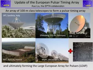
5. Major Pulsar Timing Array Projects • European Pulsar Timing Array (EPTA) • Radio telescopes at Westerbork, Effelsberg, Nancay, Jodrell Bank, (Cagliari) • Normally used separately, but can be combined for more sensitivity • Timing 23 millisecond pulsars, data spans 5 - 18 years • North American pulsar timing array (NANOGrav) • Data from Arecibo and Green Bank Telescope • Timing 40 millisecond pulsars, data spans 1 - 29 years • Parkes Pulsar Timing Array (PPTA) • Data from Parkes 64m radio telescope in Australia • Timing 24 millisecond pulsars, data spans 3 – 19 years

6. The Parkes Pulsar Timing Array Collaboration • CSIRO Astronomy and Space Science, Sydney George Hobbs, Dick Manchester, Ryan Shannon, Matthew Kerr, Aidan Hotan, John Sarkissian, John Reynolds, (Mike Keith) • Swinburne University of Technology, Melbourne Matthew Bailes, Willem van Straten, (Stefan Oslowski) • Monash University, Melbourne • Yuri Levin • University of Melbourne • Vikram Ravi(Stuart Wyithe) • University of Western Australia, Perth • Linqing Wen, Xingjiang Zhu • Curtin University, Perth • Ramesh Bhat • University of California, San Diego Bill Coles • Jet Propulsion Laboratory, Pasadena Sarah Burke-Spolaor • NSSC/NAOC, Beijing • Xinping Deng, Shi Dai • Xinjiang Astronomical Observatory, Urumqi • Jingbo Wang • Southwest University, Chongqing XiaopengYou Manchester et al. (2013)www.atnf.csiro.au/research/pulsar/ppta

7. The PPTA Pulsars All (published) MSPs not in globular clusters

8. Dispersion Corrections • Uncorrected DM variations add noise to timing data • Contribute power to unmodelled signals, e.g. gravitational waves Correction for these variations is essential! DDM = 10-4 cm-3 pc DM (10-4 cm-3 pc) • PPTA observes all pulsars in three bands: 50cm, 20cm, 10cm • Best band after DM corrections used for further analysis DtDM = 212 ns at 1.4 GHz (Keith et al. 2013) MJD

9. PPTA Timing Residuals • Timing data for 22 pulsars • Data spans to 19 years • Best 1-year rms timing residuals about 40 ns, most < 1ms • Low-frequency (red) variations significant in about half of sample – some due to uncorrected DM variations in early data, e.g., J1045-4509 • Several of best-timing pulsars nearly white (e.g., J0437-4715, J1713+0747, J1909-3744)

10. Gravitational Wave Background • Most likely detectable source of GW for PTAs is background from binary supermassive black holes in distant galaxies • Simple parameterisation of characteristic strain for cosmological distribution of circular BH binaries: • Induced modulation of timing residuals has spectrum ~ f -13/3– PTAs most sensitive to signals with f ~ 1/Tspan ~ nHz • GW spectrum may be dominated by a strong individual source (Sesana 2012)

11. Limiting the GW Background • Can use auto-correlations –pulsar terms contribute power to ACF • Detection statistic: Weights: Spectral model: GW signal: Expected signal for A95 • Used six best PPTA pulsars (fPPTA=2.8 nHz) • 95% confidence limit on GW signal in data: Observed spectrum M W Fitted GW signal (A=1.2x10-15) A95 < 2.4 x 10-15 Rel. energy density WGW(fPPTA) < 1.3 x 10-9 (Shannon et al. 2013)

12. Current PPTA Limit 95% Confidence Limits Gaussian Probability of a GW signal in the PPTA data Non-gaussian Millennium First observational challenge to physical models for the GW background! Hydro sim. (Kuiler et al. 2013) (Sesana 2013) (McWilliams et al. 2012) (Shannon et al., 2013, Science)

13. TT(PPTA2011) – Relative to TAI • PPTA extended data set, 19 pulsars • Timing referenced to TT(TAI) • Clock term sampled at ~1 yr intervals • Constrained to have no quadratic or annual terms • Compared with BIPM2010 – TAI with quadratic removed PPTA BIPM2010 First realisation of a pulsar timescale with stability comparable to that of current atomic timescales! (Hobbs et al. 2012)

14. The International Pulsar Timing Array • The IPTA is a consortium of consortia, formed from existing PTAs • Currently three members: EPTA, NANOGrav and PPTA • Aims are to facilitate collaboration between participating PTA groups and to promote progress toward PTA scientific goals • There is a Steering Committee which sets policy guidelines for data sharing, publication of results etc. • The IPTA organises annual Student Workshops and Science Meetings – 2013 meetings were in Krabi, Thailand June 17-28 • The IPTA has organisedData Challenges for verification of GW detection algorithms

15. IPTA Data Sets: 50 MSPs Bands Black: 70cm Red: 50cm Green: 35cm Blue: 20cm Aqua: 15cm Red: 10cm 1984 2013

16. Future Prospects • Continuing searches will increase number of known MSPs • Very high sensitivity of FAST and SKA should allow timing of 100 – 200 weaker MSPs • Smaller telescopes will continue to have an important role – because of jitter noise, minimum useful observation time ~ 30 min Combined IPTA data sets should give a GW detection within the next 10 years FAST SKA Mid-Frequency Array 2017 2020+

18. A Pulsar Census • Currently 2302 known (published) pulsars • 2132 rotation-powered disk pulsars • 224 in binary systems • 317 millisecond pulsars • 142 in globular clusters • 8 X-ray isolated neutron stars • 21 magnetars (AXP/SGR) • 28 extra-galactic pulsars Data from ATNF Pulsar Catalogue, V1.48 (www.atnf.csiro.au/research/pulsar/psrcat) (Manchester et al. 2005)

19. Detection of Gravitational Waves • Generated by acceleration of massive objects in Universe, e.g. binary black holes • Huge efforts over more than four decades to detect gravitational waves • Initial efforts used bar detectors pioneered by Weber • More recent efforts use laser interferometer systems, e.g., LIGO, VIRGO, LISA LIGO eLISA • Two sites in USA • Perpendicular 4-km arms • Spectral range 10 – 500 Hz • Initial phase now operating • Advanced LIGO ~ 2016 • Orbits Sun, 20o behind the Earth • Two or three spacecraft • Arm length 5 million km • Spectral range 10-4 – 10-1 Hz • Planned launch ~2028

20. The Isotropic GW Background • Strongest source of nHz GW waves is background from orbiting super-massive black holes in distant galaxies Rate of energy loss to GW: Chirp mass: Frequency in source frame: • Number of mergers per comoving volume based on model for galaxy evolution (e.g. Millennium simulation) plus model for formation and evolution of SMBH in galaxies (Sesana 2013)

21. distSimpleparameterisation of characteristic strain for cosmological ributionof circular BH binaries: A is the characteristic strain at a GW frequency f = 1/1 yr • GW modulates observed pulsar frequency • Modulation spectrum of observed timing residuals: GW power ~ f -13/3 • Pulsar timing arrays are most sensitive to GW signals with frequency f ~ 1/Tspan~ few nanoHertz • Strength of GW background often expressed as a fraction of closure energy density of the Universe: (Phinney 2001; Jenet et al. 2006)

22. Stochastic GW Background: Distribution of SMBBH • Most of background from SMBBH in galaxies at z = 1-2 • Biggest contribution from largest BH masses: 108 – 109Msun (Sesana et al. 2008)

23. Localisation of GW Sources • Fits quadrupolar signature to arbitrary waveforms for multiple pulsars – good for continuous or burst sources • Strong GW source injected into PPTA data sets • Grid search over sky to measure detection significance as function of position • “Blind” search: independent software for injection and detection Source detected at close to correct position (George Hobbs and Ryan Shannon)

24. The Gravitational Wave Spectrum

25. DM Correction • Observed ToAs are sum of frequency-independent “common-mode” terms tCM(e.g., clock errors, GW, etc) and interstellar delays tDM – assume ~ l2 • The interstellar term tDM is noise – want to minimise it • Observe at ~zero wavelength, i.e., X-ray or g-ray • Observe at two or more wavelengths, l1 and l2 (with l1 > l2) • Can then solve for tDM and tCM:

26. Effect of CM Term No CM Pre-fit (Wh+GW+DM) • If CM term not included in fit, power is extracted from freq-independent variations and coupled into DM variations • With CM term included, all freq-independent power (e.g., GW signal, clock errors) is contained in CM values Pre-fit (Wh+GW) Post-fit 1 yr-1 10 yr-1 CM incl. (Keith et al. 2013) Power spectra of timing residuals

27. MSP Polarisation • Grand-average profiles for PPTA pulsars, very high S/N • New profile features, complex polarisation properties (Yan et al. 2010)

28. Pulsars as Clocks • Because of their large mass and small radius, NS spin rates - and hence pulsar periods – are extremely stable • For example, in 2001, PSR J0437-4715 had a period of : 5.7574519243621370.000000000000008 ms • Although pulsar periods are very stable, they are not constant • Pulsars are powered by their rotational kinetic energy • They lose energy to relativistic winds and low-frequency electromagnetic radiation (the observed pulses are insignificant) • Consequently, all pulsars slow down (in their reference frame) • Typical slowdown rates are less than a microsecond per year • For millisecond pulsars, slowdown rates are ~105 smaller

29. Measurement of pulsar periods • Start observation at a known time and average 103 - 105 pulses to form a mean pulse profile • Cross-correlate this with a standard template to give the arrival time at the telescope of a fiducial point on profile, usually the pulse peak – the pulse time-of-arrival (ToA) • Measure a series of ToAsover days – weeks – months – years • Transfer ToAsto an inertial frame – the solar system barycentre • Compare barycentricToAswith predicted values from a model for the pulsar – the differences are called timing residuals. • Fit the observed residuals with functions representing errors in the model parameters (pulsar position, period, binary period etc.). • Remaining residuals may be noise – or may be science!

30. Sources of Pulsar Timing “Noise” • Intrinsic noise • Period fluctuations, glitches • Pulse shape changes • Perturbations of the pulsar’s motion • Gravitational wave background • Globular cluster accelerations • Orbital perturbations – planets, 1st order Doppler, relativistic effects • Propagation effects • Wind from binary companion • Variations in interstellar dispersion • Scintillation effects Pulsars are powerful probes of a wide range of astrophysical phenomena • Perturbations of the Earth’s motion • Gravitational wave background • Errors in the Solar-system ephemeris • Clock errors • Timescale errors • Errors in time transfer • Instrumental errors • Radio-frequency interference and receiver non-linearities • Digitisation artifacts or errors • Calibration errors and signal processing artifacts and errors • Receiver noise

31. PSR J0730-3039A/B The first double pulsar! • Discovered at Parkes in 2003 • One of top ten science break-throughs of 2004 - Science • PA = 22 ms, PB = 2.7 s • Orbital period 2.4 hours! • Periastron advance 16.9 deg/yr! (Burgay et al., 2003; Lyne et al. 2004) Highly relativistic binary system!

32. Measured Post-Keplerian Parameters for PSR J0737-3039A/B GR value Measured value Improves as  Periast. adv. (deg/yr) - 16.8995  0.0007 T1.5  Grav. Redshift (ms) 0.3842 0.386  0.003 T1.5 Pb Orbit decay -1.248 x 10-12 (-1.252  0.017) x 10-12 T2.5 r Shapiro range (s) 6.15 6.2  0.3 T0.5 s Shapiro sin i 0.99987 0.99974 T0.5 . . +16 -39 GR is OK! Consistent at the 0.05% level! Non-radiative test - distinct from PSR B1913+16 (Kramer et al. 2006)