Clustering on Local Appearance for Enhanced Deformable Model Segmentation in CT Imaging
190 likes | 320 Vues
This study presents a novel approach to deformable model segmentation of bladder and prostate tissues in CT imaging by utilizing clustering on local appearance features. Recognizing the challenges posed by low contrast and variability in CT scans, we explore a Bayesian deformable model approach that engages local intensity distributions. Through extensive experiments on a dataset of 5 patients, we demonstrate that local clustering leads to segmentations that closely match expert segmentations, offering a promising direction for radiation treatment planning and improving segmentation quality.

Clustering on Local Appearance for Enhanced Deformable Model Segmentation in CT Imaging
E N D
Presentation Transcript
Clustering on Local Appearance for Deformable Model Segmentation Joshua V. Stough, Robert E. Broadhurst,Stephen M. Pizer, Edward L. Chaney MIDAG, UNC-Chapel Hill ISBI 2007, SA-AM-OS2b April 14, 2007
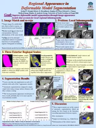
Problem: Bladder and Prostate in CT • Low contrast • Variability across days.
Clustering on Local Appearance for Deformable Model Segmentation • Bayesian Deformable Model Segmentation • Appearance / Image Match • Clustering on Local Appearance • Results on bladders and prostates in CT • Conclusions
Deformable Model Segmentation (DMS) for Radiation Treatment Planning • Segmentation is challenging and high cost for clinicians. • Bayesian DMS • Image match trained on expert segmentations
Deformable Model and Locality • M-rep provides: • Boundary rep. with normals • Correspondence • Statistical deformation p(m) • p(I | m), image match • We consider appearance at local patches. [Pizer et al., IJCV 55 (2) 2003][Fletcher et al., TMI 23 (8) 2004] Atom grid Implied Surface
Image Match p(I|m): Related Work • Profile-based, voxel-scale correspondence • AAM, [Cootes et al., CVIU 61 (1) 1995] • AAM +, [Scott et al., IPMI 2003] • Intensity Profile Clustering, [Stough et al., ISBI 2004] • Region-based • Intensity Ranges, [Zhu et al., PAMI 18 (9) 1996] • Summary Statistics • [Tsai et al., TMI 22 (2) 2003] • [Chan et al., TIP 10 (2) 2001] • Histogram Metrics • [Rubner et al., CVIU 84 2001] • [Freedman et al., TMI 24 (3) 2005] • Statistics on Distributions, [Broadhurst et al., ISBI 2006]
Appearance: Regional Intensity Quantile Functions (RIQFs) [Levina, UC-Berkeley 2002] [Broadhurst et al., ISBI 2006] • Inverse cumulative distribution function. • Suited to PCA. • Regional – local object-relative image extent. • Example: probability density and quantile function.
Global regions Versus geometrically defined local regions Versus regions defined by RIQF clusters. Question: Which Image Match Produces Best Segmentations?
Determine Region Types • Pool RIQFs over all regions and training images. • Fuzzy C-Means Clustering • Example: C= 2 on bladder exterior. [Bezdec 1981]
Eig. 2 Z-score Eig. 1 Z-score Partition the Boundary by Cluster Type • For each patch, choose most popular cluster. • PCA on cluster populations.
Bladder Partition for C= 2 • Confirming evidence • Bladder: mostly fat with prostate and bone • Prostate: dense tissue with bone and bladder, some fat
Experimental Setup Determine local RIQF-types in training data Construct Gaussian models on each type Build a template of optimal types • 5 patient image sets, ~16 images per patient. • UNC RadOnc and William Beaumont, Michigan. • 512 5120.98 0.98 3 mm
Results Summary, Global v Clustered RIQF clustered image match compares favorably with global.
Conclusions: • Local-clustered regions lead to improved segmentations • Already approaching expert quality, exceeding agreement between experts. Future Directions: • Improved clustering • Modeling mixtures • Region shifting
A walk in the projected space of local intensity distributions
Cluster statistics are not specific enough. • Evidence for modeling each patch separately.