Force-Directed Methods

1. Force-Directed Methods — Drawing Undirected Graphs

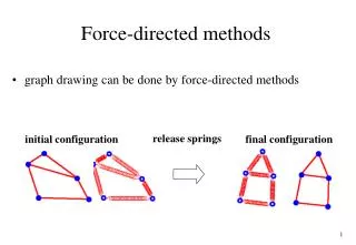
2. Force-Directed Methods • Use a physical analogy to draw graphs • How does the natural “draw” a graph? • View a graph as a system of objects with forces acting between them. • Assumption: a balanced system gives a good layout • Specifically, a system configuration with locally minimal energy: • The sum of the forces on each object is zero.

3. Force-Directed Methods • Vertex: • Object of the system; • Interacting with each other based on “some” force(s). • Edge: • A different type of object; • Not interacting with each other; • Add new force(s) to vertex object. • Equilibrium configuration: the sum of forces on each vertex object is zero

4. There are many force directed methods. In general, they have two parts: model & algorithm • The model: a force system defined by vertices & edges • The algorithm: a technique for finding an equilibrium state, that is the sum of the forces on each vertex is zero (force system);or • a technique for finding a configuration with locally minimal energy (energy system)

5. Spring Methods • Vertex: • Electrically charged particles; • Repel each other. • Edge: • Spring that connect particles; • Attraction force when longer than the natural length; • Repulsion force when shorter than the natural length. 1. 2.

6. A Larger Example © Sander

7. Many Variations • Spring & electrical force • Barycenter method • Force simulating graph theoretic distance • Magnetic field • General energy function • Constraints

8. (u,v) (u,v) VxV E 1. Springs & Electrical Forces • Use a combination of spring & electrical forces • Edge: modeled as spring • Vertex: equally charged particles which repel each other • The force on v : F(v) = Σ f u,v + Σ g u,v • f u,v: force on v by the spring between u an v : follow Hook’s law (proportional to the difference between the distance between u and v and the zero-energy length of the spring) • g u,v : Electrical repulsion exerted on v by vertex u : follow inverse square law

9. d(p,q) : Euclidean distance between points p and q • pv = (xv, yv): position of vertex v • x component of the force on v lu,v: natural (zero energy) length of the spring between u and v : if the spring has natural length lu,v, no force is exerted; k1u,v : stiffness of the spring between u and v : the larger k1u,v, the more tendency for the distance between u and v to be close to lu,v. k2u,v : the strength of the electrical repulsion between u and v

10. Aim of the force model design: • Spring force: • Ensure the distance between adjacent vertices u and v is approximately equal to lu,v. • Electrical force: • Ensure vertices not too close to each other. • One may choose parameters luvk1u,v k2u,v to customize for specific applications.

11. There are many technique to find an equilibrium configuration (or minimum energy). • Simple algorithm • Initially at random location • At each iteration: • Force F(v) on each vertex is computed • Each vertex v is moved in the direction of F(v) by a small amount proportional to the magnitude of F(v) • Stops when equilibrium is achieved or some conditions are met. • Not the fastest, but allow smooth animation. • Calculating attractive forces only between neighbors: O(|E|) • Calculating repulsive forces between all pair of vertices: O(|V|2) • Bottleneck of the algorithm in general

12. Spring Embedder [Eades84] “Logarithmic spring” • Rather than Hook’s law, the spring force is calculated as: • Hook Law (linear) spring is too strong when the vertices are far

13. Advantages • Relatively simple & easy to implement • Good flexibility • Heuristic improvements easily added • Handle domain constraints • Smooth evolution of the drawing into the final configuration helps preserving the user’s mental map • Can be extended to 3D • Often able to display symmetries • Works well in practice for small graphs with regular structure • Show some clustering structure

14. Disadvantages • Slow running time • Results are acceptable, but not brilliant • Few theoretical results on the quality of the drawings produced • Difficult to extend to orthogonal & polyline drawings • Limited constraint satisfaction capability

15. 2. Barycenter Method [Tutte60,63] • Use springs with natural length 0, and attractive force proportional to the length • Pin down the vertices of the external face to form a given convex polygon (position constraint) • Let the system go…

16. luv = 0, k1u,v = 1, no electrical force • Trivial solution pv = 0 for all v

17. Partition V into two sets: fixed vertex (at least 3, nailed down) and free vertex • To achieve equilibrium, choose pvso that Fx(v) = 0 for all free vertices; • Similarly, choose pvso that Fy(v) = 0 for all free vertices. Therefore, • Where deg(v) is the degree of v, • N0(v): set of fixed neighbor of v; • N1(v): set of free neighbor of v.

18. The equations are linear. • The number of equations and the number of unknownvariables are both equal to the number of free vertices. • Solving them equals to placing each free vertex at the barycenter of its neighbours. • So the name ‘barycenter method’.

19. (u,v) (u,v) E E Algorithm Barycenter-Draw Input: partition of V, V0: at least 3 fixed vertices V1: set of free vertices Strictly convex polygon P with V0 vertices Output: position pv 1. Place each vertex u in V0 at a vertex of P and each free vertex at the origin 2. Repeat For each free vertex v do xv = 1 Sxu deg(v) yv = 1 Syu deg(v) Until xvand yv converge for all free vertices v _____ _____

20. An Example

21. 3. Force Simulating Graph Theoretic Distance [Kamada Kawai 89] • Model graph-theoretic distance with Euclidean distance • The forces try to place vertices so that their geometric distance in the drawing is proportional to their graph theoretic distance • For each pair of vertices (u, v), δ(u,v) is the graph-theoretic distance between them; • Number of edges on a shortest path between u and v. • Aim: find a drawing such that for each pair of vertices, the Euclidean distance d(pu, pv) is approximately proportional to δ(u,v) • i.e. system has a force proportional to d(pu, pv)- d(u,v)

22. E u v • Potential energy in the spring between u and v: ½ kuv (d(pu, pv) - d(u,v))2 • Choose stiffness parameter: springs between vertices that have small graph theoretic distance are stronger kuv = k / d(u,v)2 • Thus, energy in (u, v): h = k/2 (d(pu, pv)/d(u,v) – 1)2 • Energy in the whole drawing is the sum of individual energies: h = k/2 S (d(pu, pv)/d(u,v) – 1)2 • Algorithm seek a position pv=(xv, yv), for each vertex v to minimize h • h / xv = 0, h / yv = 0, v V : non linear equation • Partial derivatives with respect to each xv and yv are zero

23. However, iterative approach can solve the equation • At each step, a vertex is moved to a position that minimizes energy, while other vertices remain fixed • Choose a vertex that has the largest force acting on it, that is is maximized for all v in V.

24. 4. Magnetic Fields [SM95] • Variations: • Some or all of the springs are magnetized • There is a global magnetic field that acts on the spring • Magnetic field can be used to control the orientation of edges • 3 types of magnetic fields • Parallel: all magnetic forces operate in the same direction • Concentric: the force operates in concentric circles • Radial: the forces operate radially outward from a point

25. The three basic magnetic fields can be combined • encourage orthogonal edges with a combination of parallel forces in the horizontal & vertical directions • The springs can be magnetized in two ways: • Unidirectional: the spring tends to align with direction of the magnetic field • Bidirectional: the spring tends to align with the magnetic field, but in either direction • A spring may not be magnetized at all

26. Unidirectional magnetic spring θ Direction of the magnetic field • The magnetic field induces a torsion or rotational force on the magnetic springs. • For a unidirectionally magnetized spring representing (u,v), the force is proportional to d(pu, pv)aq b d(pu, pv): Euclidean distance between puandpv • q: angle between the magnetic field and the line from putopv • a and b are constant

27. The magnetic forces are combined with the spring & electrical force • Algorithm to find equilibrium: • initially random position and at each iteration move the vertex to lower energy position • Can handle directed graphs (unidirectional springs with one of the 3 fields) • arcs point downward: downward parallel field • Outward: radial field • Counterclockwise: concentric field • Can be applied to orthogonal drawings: combined vertical & horizontal field with bidirectional springs • Applied with success to mixed graphs (graph with both directed & undirected edges)

28. Two Examples Vertical and horizontal magnetic field Vertical magnetic field

29. 5. General Energy Function • Most of the energy function h is a simple continuous function of the location of vertices. However, many of aesthetic criteria are not continuous • Including discrete energy function • The number of edge crossings • The number of horizontal & vertical edges • The number of bends in edges • general energy function h = l1 h1 + l2 h2 + … + lk hk • hi : a measure for an aesthetic criterion • May include spring, electrical, magnetic energy

30. [Davidson & Harel 96] energy function for straight line drawings • = l1 h1 + l2 h2 + l3 h3 + l4 h4 h1= Su,v V (1/ (d(pu, pv))2 ) : similar to electrical repulsion (vertices do not come too close together) ru, lu, tu, bu: Euclidean distance between vertex u and the four side lines of rectangular area (vertices do not come too close to the border of the screen) h3= S(u,v) E (d(pu, pv))2 : edges do not become too long h4 : the number of edge crossings in the drawing

31. Flexibility of general energy function: allow variety of aesthetics by adjusting li • [BBS97]: user can choose & adjust system parameters • [Mendonca94]: how these coefficients can be automatically adjusted to user’s preference • Main problem: computationally expensive to find a minimum energy state (very slow) • simulated annealing [DH96]….. • Genetic algorithm [BBS97]… • Flexibility ensures popularity

32. [Davidson & Harel 96] simulated annealing • Energy function takes into account vertex distribution, edge-lengths, and edge-crossings • Given drawing region acts as wall • Simulated annealing: flexible optimization technique • Efficiency: very slow • 30 nodes and 50 edges • Able to deal with optimization problem in a discrete configuration space • Aim: to minimize (or maximize) the cost function

33. Using 3 different energy functions

34. 6. Constraints • Force-directed methods can be extended to support several types of constraints 6.1. Position constraints 6.2. Fixed-subgraph constraints 6.3. Constraints that can be expressed by force or energy function

35. assign to a vertex a topologically connected region where the vertex should remain Single point: a vertex nail down at a specific location Horizontal line: group of vertices arranged on a layer A circle: set of vertices to be restricted to a distinct region [Ostry96]: constraints vertices to curves and 3D surfaces 6.1. Position constraints

36. 6.2. Fixed subgraph constraints • Assign prescribed drawing to a subgraph . • May be translated or rotated, but not deformed. • Considering the subgraph as a rigid body. • For example, barycenter method is a force-directed method that constrains a set of vertices (fixed external vertices) to a polygon.

37. 6.3. Constraints expressed by forces • Constraints expressed by forces • Orientation of directed edges: magnetic spring • Geometric clustering of special set of vertices • Alignment of vertices • Clustering can be achieved [ECH97] • For each set C of vertices, add a dummy attractor vertex vC • Add attractive forces between an attractor vC and each vertex in C. • Add repulsive forces between pairs of attractors and between attractors and vertices not in any cluster.

38. Remark • Improve the efficiency • [FR91]: amenable force functions • [FLM95, Tun92]: use randomization in S.A. • [Ost96]: the equations describing the minimal energy states are stiff for some graphs of low connectivity. • [HS95]: use combinatorial preprocessing step, good initial layout • [BHR96] empirical analysis • [FR91],[KK89],[DH96],[Tun92],[FLM95] • No winner, try several methods and then choose the best

39. Faster Spring methods • Problem: Spring methods are too slow for huge graphs 1.pu = some initial position for each node u; 2. Repeat • 2.1Fu := 0 for each node u; • 2.2For each pair u,v of nodes 2.2.1 calculate the force fuv between u and v; 2.2.2Fu += fuv; 2.2.3Fv += fuv; • 2.3For each node u, pu += eFu; Untilpu converges for all u; Computing the forces takes quadratic time

40. Clustered Graph Graph FADE [Quigley & Eades01] • It is feasible to use • a spring method, then • a geometric clustering method to obtain a good graph clustering.

41. A tree data structure Each internal node has up to four children. Most often used to partition a two dimensional Recursively subdividing it into four quadrants or regions. Stops when each quadrant contains one point. In general, recursively partition the space into 2d subspace equally, where d is the dimension Known as Octree for 3D Quadtree

42. c BR TL a b d BL e f Barnes-Hutt method • A method of computing forces between stars. • Use Quadtree to cluster the stars • Use the forces between the clusters to approximate the forces between individual stars. root a b d c e f

43. s c BR TL a b d BL s e f Barnes-Hutt method • The contents of a subtree of can be approximated by a mass at the centroid. root a b d c e f

44. c s BR TL a b d BL s e f Barnes-Hutt method • The force that the subtree s exerts on the star x can approximate the sum of the forces that the nodes in s exert on x. root a b d c e f

45. FADE To compute the force on star x, we proceed from the root toward the leaves. ComputeForce(star x; treenode t) If the approximation is good then return the approximation; else return SsComputeForce(x, s), where the sum is over all children s of t. A simple method can be used to determine whether the approximation is good; it depends on the mass of nodes and the distance between x and s. w(t) / d(x,t) < c, w(t) the width of t; d(x,t) the distance between x and t, and c is a constant.

46. FADE • The Barnes-Hutt method is faster than the usual spring algorithm. 1.px = some initial position for each star x; 2. Repeat 2.1 Build the quadtree; 2.2Foreach star x ComputeForce(x,root); 2.3Foreach star x, px += eFx; Untilpx converges for all x; In practice, computing all the forces takes O(n log n) time

47. FADE • At each iteration, the node movements introduced in the previous step improves the quadtree clustering • Makes the quadtre clustering (a geometric clustering) better reflects the graph clustering. 1.pu = some initial position for each node u; 2. Repeat 2.1 Build the quadtree; 2.2Foreach node u ComputeForce(u,root); 2.3Foreach node u, pu += eFu; Untilpu converges for all u; Some nodes migrate from one cluster to the next

48. FADE • Observations • The Quadtree provides a clustering of the data • If the data is well clustered, then BH runs faster • The approximated force is then more accurate • The spring algorithm tends to cluster the data • This means that we can: • Use Barnes-Hutt to compute the clusters as well as the drawing • Use the quadtree as the clustering for the clustered graph

49. Experimental Result The error is the difference between the approximated force vector and the original one Visual abstraction

50. Can we use other natural system analogy?