Download
1 / 37
380 likes | 481 Vues
Explore the optical interferometry method using the VLTI instrument MIDI to study asteroids. Understand visibility, coherence, and source size measurements. Learn about the VLT Interferometer's AMBER and MIDI instruments and their observational capabilities. Discover the advantages and technical challenges of using interferometry in space research. Gain insights into the complex visibility calculations and maximizing data accuracy through proper baseline sampling. Uncover the potential of binary systems observations and the VLT Interferometer's powerful capabilities.

E N D
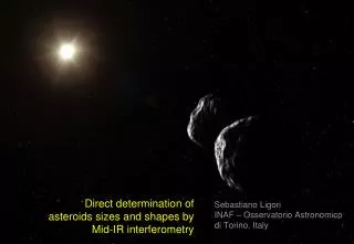
Direct determination of asteroids sizes and shapes by Mid-IR interferometry Sebastiano Ligori INAF – Osservatorio Astronomico di Torino, Italy
Overview • What is optical interferometry, advantages and technical challenges • The 10 micron instrument at the VLTI: MIDI • First successful observations of asteroids with MIDI • Lessons learned and future prospects
A schematic view of an optical interferometer An interferometer needs a number of active components, from the traditional adaptive optics to the delay lines for tracking the change in Optical Delay during the observations, to a fast fringe tracking system to compensate for the effect of turbulence on the incoming wavefront.
[ImaxImin] V = [Imax+Imin] The observable: visibility The quantity that can be determined in an interferometer is the modulus of the Visibility, and is basically the contrast of the interferometric fringe. The complex visibility is determined also by the phase, i.e. the position of the white light fringe. The complex visibility is related to the coherence function of the source.
The effect of spectral width The output of a 2 telescope interferometer for a point source is, at a given wavelength, a sine wave: The maxima are separated by an integer number of wavelengths. The superposition of many wavelengths reduces the coherence of the interferometry pattern.The coherence length is defined by coh = 20/
The link between visibility and source size The visibility measurements give information on the source luminosity distribution at a given spatial frequency. The Van Cittert-Zernicke theorem states in fact that, defining the spatial frequency components u=Bx/l and v=By/l, the complex visibility is given by V(u, v) = I(l, m) ei2(ul + vm) dl dm I(l, m) dl dm In order to properly sample the u,v space one needs to adopt several baselines with different length and orientation. Using the earth rotation it is possible to obtain several baseline with the same pair of telescopes. In any case good u,v sampling can be very time consuming. If the source can be approximated by a simple model, a smaller number of baselines can give valuable information.
Uniform disk The simplest model for the brightness distribution of an object (apart from a point source) is the uniformly illuminated disk. In order to have a good signal to noise, one should sample the visibility curve in the region where the visibility is still relatively large. However, deviations from the simple model (for instance in the case of limb darkening) will be more evident near the first minimum
Binary systems • When a binary is unresolved by the single telescope, the measured visibility will depend on the luminosity ratio, diameter and separation of the two components • In the case of two point source we have the following expression: While, more in general
The Very LargeTelescope Interferometer • Located on Cerro Paranal, Chile, 2600 m • Low humidity, very good for Mid-IR observations • 4 Unit Telescopes (8m) • 4 Auxiliary Telescopes (1.8m) • Baselines ranging from 8 to almost 200 m
AMBER • Amber is the near-IR instrument of the VLTI It is a three beam instrument, which allows to obtain visibilities and phase information, therefore making it possible to synthesize images. Due to the low efficiency, imaging capabilities are quite limited.
AMBER raw data Combination of three beams Photometric beams
The 10 micron instrument of the VLTI: MIDI • MIDI combines two beams and works in the thermal IR (8-13 micron)
MIDI:high background observations As any Mid-IR instrument from the ground, MIDI is affected by a high and variable background from the sky, the telescopes and all the optics in the tunnel. To get the photometric information on our target, we need to apply the usual chopping technique (simultaneously on both telescopes).
The MIDI signal: dispersed fringes • Since in MIDI the beam combination is performed at the pupil, the result on the focal plane is the (dispersed) image of the target as seen by the single telescope, with a flux modulation obtained by changing the local OPD. The dispersed fringes can be used to deduce where the exact optical equalization occurs; the farther we are from zero OPD, the larger is the number of fringes we can see in the spectrum.
Two observing modes High Sensitivity mode:Fringe tracking: exclusively on the source, no chopping2 windowsPhotometry for each telescope is obtained by closing a the shutter of the other beam, with beam combiner inserted and chopping2 windows located at the same place in the detectorAdvantage: simple data sets in the same detector positionDrawback: Photometry performed at 2-5 minutes intervals. The accuracy on the visibility is typically 7-15% under good to medium atmospheric conditions, Science Photometry modeFringe tracking: chopping working at a frequency which is an integer mulitplier scanning of the scanning frequency4 windows: 2 interferometric, 2 photometricAdvantage: simultaneous photometryDrawbacks: chopping simultaneously with scanning, heavy real time control : distorsion of the photometric beams, added detector noise
Preparing the observations • In order to apply for observing time at ESO, one needs to demonstrate feasibilty; therefore, to show that the combination of flux and (expected visibility) is above the detection threshold one can run a simulation of the target. ESO provides a tool (VisCalc: http://www.eso.org/observing/etc/) that allows one to select the right baseline and HA of observation. Binary system Separation 70 mas PA 12 Diameter 40 mas / 30 mas MIDI, with UT2 – UT3 and UT3 – UT4 baselines
Preparing the observations: Calibrators • There is a loss of coherence due to instabilities in the instrument and to the atmospheric characteristics • Need to calibrate with a source with known visibility, possibly with high SNR, as close as possible to our target • An ESO resource (Calvin, see http://www.eso.org/observing/etc/ ) helps looking for the right calibrator. • It can be a hard task, especially with the ATs!
Scientific applications The main application of interferometry has been for a long time determinining stellar diameter; a number of applications emerged in recent years: • Dust disks around young stars • Massive stars • Planetary nebulae, symbiotic systems • AGNs • Binary systems (in case of double lined spectroscopic binaries: mass determination)
Scientific applications Recently, closure phase on several baselines has been used on AMBER to get the first real images on T Lep: see ESO PR 06/09
Determining asteroid diameters • Thermal models are able to derive the asteroid size by measuring the thermal emission • Since log pV = 6.247 − 2 logD − 0.4H , normally one can use knowledge of the magnitude and assumptions on the albedo (e.g. derived from polarimetric measurements) to determine the Diameter D • The only direct method so far makes use of stellar occultation, but of course this method is limited by the narrow window of observability and by uncertainty of stellar catalogues and asteroids' orbital elements • With inteferometry we get a direct measurement, in particular for spherical objects. Objects with peculiar shapes need a larger number of visibility points
Asteroid observations with MIDI • Normally the diameter of asteroids can be determined only indirectly, through the apparent magnitude and an assumption on the albedo of the object. Direct methods are limited to the largest or closest objects • MIDI observations of asteroids allow us to get direct information on size and shape of the asteroids, and to obtain this information for a range of wavelengths • At the same time, we obtain low resolution spectra of these objects • The combination of diameter size, shape and spectrum can be compared with different thermal models of the objects. As we shall see, MIDI observations allow us to discriminate between different models
Limitations of the interferometric method • The main limitation is related to the sensitivity of the instrument to the fringe contrast that can be measured; this is expressed in terms of "correlated flux", that is the flux of the object multiplied by the visibility. • Larger object can have higher fluxes but are also larger and the visibility drops; fringe measurements can be made if the correlated flux is larger than 1 Jy at 10 micron (actually 0.2 Jy have been observed) • Observations of targets with relatively large diameters can be observed with the ATs, using a short baseline (e.g. 16 meters); in this case the limiting correlated flux for MIDI is about 20 Jy • ATs are also providing the longest baselines on the VLTI, so they are useful to resolve very compact objects
Asteroids observable with MIDI • Diamonds: MBAs. • Squares:NEAs
MIDI observations of asteroids: first success • An initial try with 1459 Magnya has not been successful; the observations were made during VLTI SDT and adopted a 100 m baseline, giving a small visibility on an already faint (less than 1 Jy) object (Delbo et al, Icarus 181, 618, 2006) • First success: observations of 951 Gaspra and 234 Barbara (Delbo et al., 2008, accepted on ApJ).The team is composed by M. Delbo and A. Matter (Obs. Cote d'Azur, Nice), S. Ligori and A. Cellino (OATo); and J. Berthier (Institut de Mecanique Celeste, Paris) • Gaspra can be considered a "test" object; it has been flown by during the Galileo mission, so that diameter and shape are quite well known • Barbara belongs to a taxonomic group characterized by peculiar polarimetric properties, so that polarimetry cannot be used to infer the albedo and the diameter
The observations • Both targets have been observed combining the light from UT2 and UT3, with a baseline of about 47m. The baseline projected on the sky depends on the coordinates of the target and on the HA at observation.
Results: Gaspra • Using the knowledge of the shape of Gaspra, one can determine the orientation of the baseline with respect to the target, and make predictions on the visibility one should obtain.
Thermal models • The diameters of asteroids can be derived, from the Mid-IR thermal emission, using models that simulate the thermal characteristics of the body in terms of thermal inertia and roughness. • From the MIDI spectra, we derived the diameters of the two targets using the Standard Thermal Model (STM, Lebofsky et al. 1986), the Near Asteroids Thermal Model (NEATM, Harris 1998), and the Fast Rotating thermal Model (FRM, see Harris and Lagerros 2002; Delbo and Harris 2002) • The derived diameters were used to produce the expected visibilities, to be compared with our MIDI data
Gaspra • In this case the object is almost unresolved. NEATM and STM fit both the visibility and the observed spectrum; the diameter, derived from the uniform disk model, is 17 mas, corresponding to 11 km. STM = Standard Thermal Model NEATM = Near Earth Asteroids Thermal Model FRM = Fast Rotating thermal Model
Barbara • In this case the best fit to the visibility is given by a "binary" formula, while the sizes derived with the thermal models do not fit at all the observed behaviour, even if they fit well (except FRM) the spectrum. This is due to the peculiar shape of the target.
Barbara • The observed visibility can be interpreted as a binay, but with a single measurement is not possible to get all the information we need on the separation Primary: 43 mas (37 km) Secondary 24 mas (21 km) Separation: 28 mas (24 km)
Conclusions and Future prospects • The interferometric technique proved to be feasible and accurate; the VLTI infrastructure can now work routinely on moving targets • Constrains in correlated flux are the main limitation; availability of visibility calibrators when using the ATs also an issue • It is absolutely necessary to get several visibilities points per object, in particular to investigate non spherical shapes and/or binarity • Thermal models do a good job in determining diameters, in "normal" cases • Add more objects, possibly more baselines on objects already observed • Some new data already available, on Victoria and Daphne, more are coming