Download
1 / 10
100 likes | 365 Vues
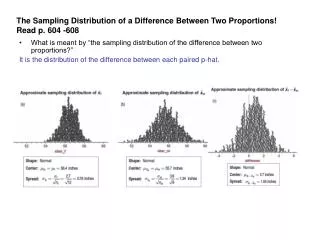
The Sampling Distribution of a Difference Between Two Proportions! Read p. 604 -608. What is meant by “the sampling distribution of the difference between two proportions?” It is the distribution of the difference between each paired p-hat.

E N D
The Sampling Distribution of a Difference Between Two Proportions!Read p. 604 -608 • What is meant by “the sampling distribution of the difference between two proportions?” It is the distribution of the difference between each paired p-hat.
What are the shape, center, and spread of the sampling distribution of ? Are there any conditions that need to be met? Shape: When n1p1,n1 (1 – p1), n2p2, and n2(1 – p2) are all at least 10, the sampling distribution of is approximately Normal. Center: The mean of the sampling distribution is . That is, the difference in sample proportions is an unbiased estimator of the difference in population proportions. Spread: the standard deviation of the sampling distribution of is As long as each sample is no more than 10% of its population. What does the standard deviation of the sampling distribution of measure? When samples are taken many many times, the standard deviation tells us how far the difference in the sample populations will be from the true difference in proportions, on average.
-.065 0 .065 -.13 .13 • Example: • Suppose that two counselors at School 1, Michelle and Julie, independently take a random sample of 100 students from their school and record the proportion of students who did their homework last night. When they are finished, they find that the difference in their proportions, , is 0.08. They are surprised to get a difference this big considering that they were sampling from the same population. • (a) Describe the shape, center, and spread of the sampling distribution of • Since nMpM = 70,nM (1 – pM) = 30, nJpJ = 70, and nJ(1 – pJ) = 30are all at least 10, the sampling distribution of is approximately Normal. Its mean is and its standard deviation is • (b) Find the probability of getting two proportions that are at least 0.08 apart. • We can calculate the probability that or Using technology, the probability is normalcdf(-100,-0.08,0,0.065) + normalcdf(0.08,100,0,0.065) = 0.2184
(c) Should the counselors have been surprised to get a difference this big? • Since the probability isn’t very small, we shouldn’t be surprised to get a difference of sample proportions of 0.08 or larger just by chance, even when sampling from the same population. • Confidence Intervals for p1 - p2 • Read p. 608 – 611 • What is the standard error of ? How is this different than the standard deviation of ? • What is the formula for a two-sample z interval for ? Is this on the formula sheet?
What are the conditions for calculating a two-sample z interval for ? How are these different than the conditions for a one-sample z interval for p? • Random: SRS for both populations in a randomized experiment • Normal: and • Independent: Both samples and individual observations in each group are independent. When sampling without replacement, check that the two populations are at least 10 times as large as the corresponding samples. • Is it OK to use your calculator for the Do step? Are there any drawbacks? • It is ok to use a calculator for the Do step. Just make sure you don’t choose the wrong procedure on your calculators. The 2-sampleZint is for comparing means when the population and standard deviations are known. What you want to use is the 2-PropZint. If you use the wrong feature, you will not get any credit on the “Do” step. • We recommend that you use your calculators to do the calculations and then go back and if there is time, go back and double-check your calculations when you finish the exam.
Example: • Many news organizations conduct polls asking adults in the United States if they approve of the job the president is doing. How did President Obama’s approval rating change from August 2009 to September 2010? According to a CNN poll of 1024 randomly selected U.S. adults on September 1–2, 2010, 50% approved of Obama’s job performance. A CNN poll of 1010 randomly selected U.S. adults on August 28–30, 2009, showed that 53% approved of Obama’s job performance. • (a) Explain why we should use a confidence interval to estimate the change in Obama’s approval rating rather than just saying that his approval rating went down 3 percentage points. • We expect the sample to vary somewhat from the true proportion and therefore we need an a confidence interval to estimate the true difference. • (b) Use the results of these polls to construct and interpret a 90% confidence interval for the change in Obama’s approval rating among all U.S. adults. • State: We want to estimate p2010 – p2009 at the 90% confidence level where p2010 = the true proportion of all U.S. adults who approved of President Obama’s job performance in September 2010 and p2009 = the true proportion of all U.S. adults who approved of President Obama’s job performance in August 2009. • Plan: We should use a two-sample z interval for p2010 – p2009 if the conditions are met. • Random: The data came from separate random samples. • Normal: and which are all at least 10. • Independent: The samples were taken independently and there were at least 10(1024) =10,240 U.S. adults in 2010 and 10(1010)=10,100 U.S. adults in 2009. • Do: • Conclude: We are 90% confident that the interval from -0.066 to 0.006 captures the true change in the proportion of U.S. who approve of President Obama’s job performance from August 2009 to September 2010. That is, it is plausible that his job approval has fallen by up to 6.6 percentage points or increased by up to 0.6 percentage points.
(c) Based on your interval, is there convincing evidence that Obama’s job approval rating has changed? • Since 0 is included in the interval, it is plausible that there has been no change in President Obama’s approval rating. Thus, we do not have convincing evidence that his approval rating changed between August 2009 and September 2010. • Significance Tests for p1 - p2 • Read p. 611 - 615 • What is the pooled (combined) sample proportion? Why do we pool the sample proportions? • We get a more precise estimate of p when we use more data. • What is the test statistic for a two-sample z test for a difference in proportions? Is this on the formula sheet? What does the test statistic measure? • What are the conditions for conducting a two-sample z test for a difference in proportions? Random, Normal, and Independent
Example: • Are teenagers going deaf? In a study of 3000 randomly selected teenagers in 1988–1994, 15% showed some hearing loss. In a similar study of 1800 teenagers in 2005–2006, 19.5% showed some hearing loss. (These data are reported in Arizona Daily Star, August 18, 2010.) • (a) Do these data give convincing evidence that the proportion of all teens with hearing loss has • increased? • State: we will test H0: p1 – p2 = 0 versus Ha: p1 – p2 > 0 at the 0.05 confidence level, where p1 = the proportion of all teenagers with hearing loss in 2005-2006 and p2 = the proportion of all teenagers with hearing loss in 1988-1994. • Plan: We should use a two-sample z test for p1 – p2 if the conditions are met • Random: The data came from separate random samples • Normal: 1800(.195)=351, 1800(.805) = 1449 and 3000(.15) = 450, 3000(.85) = 2550 are all at least 10 • Independent: The samples were taken independently, and there were at least 10(1800) = 18,000 teenagers in 2005-2006 and 10(3000) = 30,000 teenagers in 1988-1994. • Do: • P-value ≈ 0 • Conclude: Since the P-value is less than 0.05, we reject the null hypothesis. We have convincing evidence that the proportion of all teens with hearing loss has increased from 1988-1994 to 2005-2006. • (b) Between the two studies, Apple introduced the IPod. If the results of the test are statistically significant, can we blame IPods for the increased hearing loss in teenagers? • No. Wince we didn’t do an experiment where we randomly assigned some teens to listen to iPods and other teens to avoid listening to iPods, we cannot conclude that iPods are the cause. It is possible that teens who listen to iPods also like to listen to music in their cars, and perhaps the car stereos are causing the hearing loss.
Inference for Experiments • Read p. 615 - 619 • What mistake do students often make when defining parameters in experiments? How can you avoid it? • Many students don’t use the correct language when defining parameters, especially in experiments. P1-hat is the sample proportion and p1 is the parameter. • Can you use your calculator for the Do step? Are there any drawbacks? • If you use the 2-PropZTest to calculate the test statistic and P-value and type in a value incorrectly, you will receive no credit for the “Do” step.
Example: • In an effort to reduce health care costs, General Motors sponsored a study to help employees stop smoking. In the study, half of the subjects were randomly assigned to receive up to $750 for quitting smoking for a year while the other half were simply encouraged to use traditional methods to stop smoking. None of the 878 volunteers knew that there was a financial incentive when they signed up. At the end of one year, 15% of those in the financial rewards group had quit smoking while only 5% in the traditional group had quit smoking. Do the results of this study give convincing evidence that a financial incentive helps people quit smoking? (These data are reported in Arizona Daily Star, February 11, 2009.) • State: We will test H0: p1 – p2 = 0 versus Ha: p1 – p2 > 0 at the 0.05 significance level, where p1 = the true quitting rate for employees like these who get a financial incentive to quit smoking and p2 = the true quitting rate for employees like these who don’t get a financial incentive to quit smoking. • Plan: We should use a two-sample z test for p1 – p2 if the conditions are satisfied. • Random: The treatments were randomly assigned. • Normal: 439(.15)= 65.85, 439(.85) = 373.15, 439(.05) = 21.95, and 439(.95) = 417.05 are all at least 10. • Independent: The random assignment allows us to view these two groups as independent. We must assume that each employee’s decision to quit is independent of other employees’ decisions. • Do: • P-Value ≈ 0 • Conclude: Since the P-value is less than 0.05, we reject H0. We have convincing evidence that financial incentives help employees like these quit smoking.