Chapter 1 Basic Statistics
Chapter 1 Basic Statistics. FARAH ADIBAH ADNAN ENGINEERING MATHEMATICS INSTITUTE (IMK). CHAPTER 1. Basic Statistics Statistics in Engineering Collecting Engineering Data Data Summary and Presentation Probability Distributions - Discrete Probability Distribution

Chapter 1 Basic Statistics
E N D
Presentation Transcript
Chapter 1Basic Statistics FARAH ADIBAH ADNAN ENGINEERING MATHEMATICS INSTITUTE (IMK)
CHAPTER 1 • Basic Statistics • Statistics in Engineering • Collecting Engineering Data • Data Summary and Presentation • Probability Distributions - Discrete Probability Distribution - Continuous Probability Distribution • Sampling Distributions of the Mean and Proportion
Statistics in engineering • Statistics - area of science that deals with collection, organization, analysis, and interpretation of data. • Statistics - deals with methods and techniquesthat can be used to draw conclusions about the characteristics of a large number of data points, commonly called a populationby using a smaller subset of the entire data called sample. • Because many aspects of engineering practice involve working with data, obviously some knowledge of statistics is important to an engineer.
Specifically, statistical techniques can be a powerful aid in designing new products and systems, improving existing designs, and improving production process. • The methods of statistics allow scientists and engineers to design valid experiments and to draw reliable conclusions from the data they produce
Collecting Engineering Data • Direct observation The simplest method of obtaining data. Advantage: relatively inexpensive. Disadvantage: difficult to produce useful information since it does not consider all aspects regarding the issues. • Experiments More expensive methods but better way to produce data. Data produced are called experimental. • Surveys Most familiar methods of data collection. Depends on the response rate. • Personal Interview Has the advantage of having higher expected response rate. Fewer incorrect respondents.
Data Presentation • Data can be categorized into two :- - Qualitative data - qualitative attributes - Quantitative data - quantitative attributes • Two sources of data :- - Primary ( eg. Questionnaire, Telephone Interview) - Secondary (eg. Internet, Annual Report) Data should be summarized in more informative way such as graphical, tables or charts.
Data Presentation Data can be summarized or presented in two ways: 1) Tabular 2) Charts/graphs. Data Presentation of Qualitative Data 1) Frequency Distribution Table - represents the number of times the observation occurs in the data. Example: Ethnic Group Observation Frequency Malay 33 Chinese 9 Indian 6 Others 2
2) Charts for qualitative data are: Pie Chart : Gender Bar Chart : Ethnic Group Line Chart : Number of Sandpipers from Jan 1989 – Dec 1989
Data Presentation of Quantitative Data 1) Frequency Distribution Table – list all classes and the number of values that belong to each class.
This formula will be used to form frequency distribution table, from raw data. Class - an interval that includes all the values that fall within two numbers; the lower and upper class (class limit). Class Boundary - the midpoint of the upper limit of one class and the lower limit of the next class. Class Width/Size/Interval ,c -difference between the two boundaries of a class . Formula : C = Upper boundary – Lower Boundary Class Midpoint/Mark, x – formula: (Lower Limit + Upper Limit)/2
How to Form Frequency Distribution Table • Decide the number of classes to be used. • Determine class width: • When the number of classes are given, Class width = • When the number of classes are not given, Class width = where the number of class = • Don’t forget to always round up to the nearest whole number when dealing with class width/interval. • Any convenient number that is equal to or less than the smallest values in the data set can be used as the lower limit of the first class.
25 11 15 29 22 10 5 17 21 • 13 26 16 18 12 9 26 20 16 • 23 14 19 23 20 16 27 9 21 14 Example: The following data give the total number of iPods sold by a mail order company on each of 30 days. Construct a frequency distribution table. (Hint: 5 number classes). Solution: Number of classes = 5 Class width =
Histogram: Student’s CGPA Polygon : Student’s CGPA 2) Graph for quantitative data are: Ogive: Student’s CGPA
Data Summary Summary statisticsare used to summarize a set of observations. Two basic summary statistics are 1) Measures of central tendency - Mean - Median - Mode 2) Measures of dispersion - Range - Variance - Standard deviation
Measures of Central Tendency 1) Mean ,( ) • Mean of a sample ( ) or population ( ) is the sum of the sample data divided by the total number sample. • Mean for ungroup data is given by: Sample: Population: • Mean for group datais given by: Sample: Population: where f = class frequency; x = class mark (mid point)
Example: 1) Find the mean for the set of data 4, 6, 3, 1, 2, 5, 7. Solution: 2) Find the mean of the frequency distribution table below.
(f) (x) Solution: Therefore, the mean of frequency distribution above is:
2) Median, ( ) • Median is the middle value of a set of observations arranged in ascending order and normally is denoted by ( ). • Median for ungrouped data: - The median depends on the number of observations in the data, . - If is odd, then the median is the th observation of the ordered observations / middle value. - If is even, then the median is the average of the 2 middle values ( th observation and the th observation).
Median for grouped data / frequency of distribution. The median of frequency distribution is defined by: where, = the lower class boundary of the median class; = the size of the median class interval; = the sum of frequencies of all classes lower than the median class; = the frequency of the median class.
Example: 1) Find the median for the set of data 4, 6, 3, 1, 2, 5, 7, 3. Solution: Arrange in order of magnitude : 1,2,3,3,4,5,6,7. As n = 8 (even), the median is the mean of the 4th and 5th value. Therefore, the median is 3.5 2) Find the median of the frequency distribution table below.
Cumulative Frequency Solution: To determine median class: So, the median class falls in class 3.00 – 3.25.
3) Mode, ( ) • The mode of a set of observations is the observation with the highest frequencyand is usually denoted by ( ). Sometimes mode can also be used to describe the qualitative data. *Note: • If data set with only 1 value that occur with the highest frequency, therefore it has 1 mode and it is called unimodal data. • If data set has 2 measurements with highest frequency, therefore it has 2 modes and known as bimodal data. • If data set has more than 2 measurements with highest frequency, so the data set contains more than 2 modes and said to be multimodal data.
For ungrouped data: - Defined as the value which occurs most frequent. Example: The mode for data 4,6,3,1,2,5,7,3 is 3. • For grouped data When data has been grouped into classes and a frequency curve is drawn to fit the data, the mode is the value of corresponding to the maximum point on the curve.
- Determining the mode using formula. where = the lower class boundary of the modal class; = the size of the modal class interval; = the difference between the modal class frequency and the class before it;and = the difference between the modal class frequency and the class after it. Note: The class which has the highest frequency is called the modal class.
Example: Find mode of the frequency distribution table below. Solution:
Measures of Dispersion • The measure of dispersion/spread is the degree to which a set of data tends to spread around the average value. • It shows whether data will set is focused around the mean or scattered. • The common measures of dispersion are: 1) Range 2) Variance 3) Standard deviation • The standard deviation actually is the square root of the variance. • The sample variance is denoted by s2 and the sample standard deviation is denoted by s.
1) Range • Simplest measure of dispersion. • Apply for both group & ungroup data. Ungroup data: Formula: Range = Largest value – Smallest value Group data: Formula: Range = Largest value (class limit) – Smallest value (class limit) Example: Solution: Range = Largest Value – Smallest Value = 267, 277 – 49, 651 = 217, 626 square miles.
2) Variance, ( ) • Measures the variability in a set of data. • The variance for the ungrouped data: Sample: Population: • The variance for the grouped data: Sample: Population:
Example: The variance for grouped data : Solution:
2) Standard Deviation, ( ) • The positive square root of the variance is the standard deviation. • A larger value of the standard deviation – the values of the data set are spread relatively large from the mean. • A lower value of the standard deviation – the values of the data set are spread relatively small from the mean. • The standard deviation for the ungrouped data: Sample: Population:
The standard deviation for grouped data: Sample: Population: Example: From previous example.
exercise The final results in business statistics of 40 students are recorded as below • Present the data in frequency distribution table. • Construct a histogram • Calculate mean, median, mode, variance and std deviation.