Selection on Quantitative Traits
Selection on Quantitative Traits. Q1. Today’s topic is…. Sexual selection Heritability Linkage Equilibrium Fossil Record Hardy Weinberg exceptions. Q2. This graph represents…. Heritability Selection differential Selection gradient Directional selection Stabilizing selection.


Selection on Quantitative Traits
E N D
Presentation Transcript
Q1. Today’s topic is…. • Sexual selection • Heritability • Linkage Equilibrium • Fossil Record • Hardy Weinberg exceptions
Q2. This graph represents…. • Heritability • Selection differential • Selection gradient • Directional selection • Stabilizing selection
Q3.Candace Galen worked with which group of organisms? • Flowers • Fruit flies • Beetles • Guppies • Newts
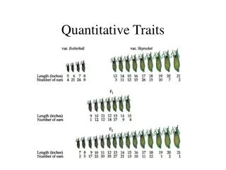
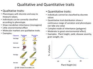
Quantitative traits are those that show continuous variation • height • skin color • plant flower size Qualitative traits are all or none • attached earlobes • widows peak • six fingers • cystic fibrosis
Quantitative genetics • provides tools to analyze genetics and evolution of continuously variable traits • Provides tools for: 1. measuring heritable variation 2. measuring survival and reproductive success 3. predicting response to selection
Measuring Heritable VariationText section 9.3 • When assessing heritability we need to make comparisons among individuals. Cannot assess a continuous trait’s heritability within one individual • Need to differentiate whether the variability we see is due to environmental or genetic differences • Heritability= The fraction of the total variation which is due to variation in genes
Types of Variation • Phenotypic variation (VP) is the total variation in a trait (VE + VG) • Environmental variation. (VE) is the variation among individuals that is due to their environment • Genetic variation (VG) is the variation among individuals that is due to their genes
Total genetic variation(VG) actually has two components • Additive Genetic Variation (VA) = Variation among individuals due to additive effects of genes • Dominance Genetic Variation(VD) = Variation among individuals due to gene interactions such as dominance • VG = VA + VD
Measuring heritability VG VG + VE VG VP • heritability = = • Heritability is always between 0 and 1 • If the variability is due to genes then it makes sense to evaluate the resemblance of offspring to their parents
Heritability can be looked at from two perspectives • Broad sense heritability = VG/ VP • Narrow sense heritability = VA / VP • We will deal only with narrow sense heritability = h2 • Use of narrow sense heritability allows us to predict how a population will respond to selection
Calculating h2- Testing the relationship between parents and offspring trait values: • Plot midpoint value for the 2 parents on x axis and mid-offspring value on y axis and draw a best fit line. • This slope which is calculated by least squares linear regression is a measure of heritability called narrow-sense heritability or h2 • h2 is an estimate of the fraction of the variation among the parentsthat is due to variation in the parent’s genes • Looking at a hypothetical population…
Figure 9.13a Pg 334 Midoffspring height Mid parent height If slope is near zero there is no resemblance Evidence that the variation among parents is due to the environment.
Midoffspring height If this slope is near 1 then there is strong resemblance Evidence the variation among parents is due to genes
Need to make sure that the environment is not causing some of the variation because “environment runs in families too.” • Any study of heritability needs to account for possible environmental causes of similarity between parent and offspring. • Take young offspring and assign them randomly to parents to be raised • In plants, randomly plant seeds in a given field • Example in text Song Sparrows studied by James Smith and Andre Dhondt.
Showed song sparrow chicks (eggs or hatchlings) raised by foster parents resembled their biological parents strongly and their foster parents not at all Figure 9.14 p. 335
Measuring differences in Survival and Reproductive Success • Done by measuring the strength of selection by looking at the differences in reproductive success. • Basically we measure who survives, who doesn’t, and then quantify the difference • Example breeding mice with longer tails
Artificial selection for long tail length • DiMasso and colleagues bred mice in order to select for longer tails • Each generation they picked the 1/3 of the mice who had the longest tails and allowed them to interbreed • Did this for 18 generations • Calculated the strength of selection
Two measures of the strength of selection • Selection differential (S) = difference between mean tail length of breeders (those that survive long enough to breed) and the mean tail length of the entire population. • Selection gradient = slope of a best fit line on a scatter plot of relative fitness as a function of tail length
Figure 9.17 p. 339 Selection differential (S) Only the 1/3 of mice with the longest tails allowed to breed (survive) Average tail length of the breeders only minus the average tail length of the entire population entire population breeders (survivors)
To calculate the selection gradient • Assign absolute fitness – fitness equals survival to reproductive age. Long tailed had a fitness of 1, short tailed a fitness of 0 • Convert absolute fitness to relative fitness. Figure the mean fitness of the population. Then divide the absolute fitness by the mean fitness. (Mean fitness = .67(0) + .33(1) = .33). So relative fitness of breeders = 1/.33 = 3.0 and relative fitness of non-breeders = 0/.33 = 0. • Make a scatterplotof relative fitness as a function of tail length. Calculate the slope using best fit. The slope is the selection gradient
Figure 9.17 p. 339 Selection gradient 1. Calculate relative fitness for each mouse, then plot relative fitness of each as a function of tail length 2. the slope of the best fit line is the selection gradient
Selection gradient is more useful because it can be used to calculate any measure of fitness not just survival • Selection differential can be calculated from selection gradient • Divide the selection gradient by the variance. Explained in box 9.3 p. 340.
Predicting Evolutionary response • Once we know the heritability and the strength of selection we can predict response to selection • R = h2S • R = predicted response • h2 = heritability • S = selection differential
Review of what we can do with the tools of quantitative genetics. • We can estimate how much variation in a trait is due to the variation in a gene (heritability) • Quantify the strength of selection that results from differences in survival or reproduction. (selection differential) • Predict how much a population will change from one generation to the next. (predicted response to selection)
Alpine skypilots and Bumblebees • Candace Galen (1966) studied the effect of selection pressure by bumblebees on flower diameter • Worked with alpine skypilots from two elevations, timberline and tundra • Tundra flowers are larger and are pollinated exclusively by bumblebees • Timberline flowers are pollinated by a mixture of insects and are smaller
Galen wanted to determine two things • Is selection by the bumblebees in the tundra responsible for the larger flower size? • How long would it take for selection pressure to increase flower size by 15%
Determining the response to selection • Determine heritability • measured flower diameters • collected seeds germinated them and transplanted seedlings to random locations in the same habitat as the parents • seven years later measured the flowers from the 58 plants which had matured enough to flower • plotted offspring flower diameter as a function of maternal (seed bearing parent) flower diameter
Analysis of results • results provided a best fit number of 0.5 for heritability. Actual calculations give h2 of 1.0 (because multiple offspring with only one parent [female]). • Scatter (fig 9.20) necessitated a statistical analysis which showed she could only be certain that at least 20% of the phenotypic variation was due to additive genetic variation. (h2 = VA / VP) Therefore h2 lies somewhere between 0.2 and 1.0
2. Determine selection differential • caged some about-to-flower Skypilotswith bumblebees • measured flower size when Skypilots bloomed and later collected their seeds • planted seedlings back out in the original parental habitat • Six years later she counted the number of surviving offspring produced by each of the parent plantsShe used the number of surviving 6 year old offspring as her measure of fitness • Plotted relative fitness (# of surviving 6 year old offspring / total number planted) as a function of maternal flower size.
Slope of best fit line is selection gradient • Calculated the selection differential (S) ( by dividing selection gradient by variance in flower size) • Her S value told her that, on average, the flowers visited by bumblebees were 5% larger than the average flower size. • Control experiments from random hand pollination and by a mixture of pollinators other than bumblebees, showed no relationship between flower size and fitness
3. Galen predicted a response • using the low end h2 of .2 and an S of .05 • R = h2S = .2 (.05) = .01 • using a high end for h2 of 1.0 and S = .05 • R = h2 S = 1(.05) = .05 • Means that a single generation of selection should produce an increase in the size of the average flower by from 1% to 5%.
Observations of a population of timberline flowers pollinated exclusively by bumblebees showed that on average flowers that were produced by bumblebee pollination were 9% larger than those pollinated randomly by hand. Galen’s prediction that response was rapid was verified
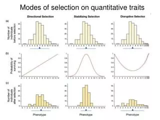
Modes of Selection on continuous traits How does each impact the distribution, fitness and survival of the possible phenotypes?
Directional Selection Examples of this type of selection are The Alpine Skypilot and the Finch beaks in times of drought. One extreme phenotypic expression of the trait increases in fitness and the other extreme decreases. • Fitness of a phenotype increase or decreases with the value of a trait. Slightly reduces the variation in a population
Stabilizing Selection • Those individuals with intermediate values are favored at the expense of both extremes. • The average value of a trait remains the same but the variation is reduced • The tails of the distribution are cut off.
Example in gall flies - Weis and Abrahamson 1986 Figure 9.26 p. 348 • A fly lays eggs in Goldenrod bud. • Plant produces a gall in response to the fly larva • Wasps lay eggs in galls that eat fly larva • Birds also eat galls. • Pressure from wasps selects for larger galls and • Pressure from birds selects for smaller galls • The result is selection for mid sized galls.
Disruptive Selection • Selects for individuals with extreme values for a trait • Does not change AVERAGE value but INCREASES phenotypic variance • Result far fewer individuals at the middle of the continuum for the trait
Example of the black-bellied seed cracker • Breeding Populations have birds with EITHER large OR small beaks • Juveniles show the full spectrum of beak size • But only the large OR small beaked birds survive to reproduce. Fiogure 9.27 p. 349
Summary • Unlike our example of the moths and other ONE gene traits…. • We are talking here about quantitative traits determined by multiple genes: • As phenotypic variation decreases so should genetic variation • However in most populations substantial genetic variation continues to be exhibited. • A satisfactory explanation for this unexpected outcome is under debate and no acceptable hypothesis is yet agreed upon.
Revisiting genetic versus environmental influences A classic experiment that opened many eyes.
Clausen Keck and Hiesey 1948 • Worked with Achillea lanulosa • On average plants from the low altitude Populations produce slightly more stems than those native to higher elevations. (30.20 to 28.32) Figure 9.31 p. 354
When grown together at low elevation, low elevation plants produced more stems This is consistent with the idea that high-altitude plants are genetically programmed to produce fewer stems
When the two source plants were grown together at high altitude …. • High altitude plants had more stems! (19.89 vs 28.32) • Each population was superior in its own environment • Apparently there are genetic differences that control how each respondsto the environment • This is a demonstration ofphenotypic plasticity
Limits of heritability studies • Must always remember that variation has both a genetic and an environmental component. • Any estimate of heritability is specific to a particular population living in a particular environment. • High heritability within groups tell us nothing about the origin of the differencesbetween groups • Cannot be usedto determine the differences between populations of the same speciesthat live in different environments.
All that we can really gain by measuring heritability is the ability to predict whether selection on the trait will cause a population to evolve