Quantitative and Polygenic Traits
http://biolmolgen.slam.katowice.pl/. Quantitative and Polygenic Traits. Aleksander L. Sieroń Dep artmen t of General and Molecular Biology and Genetics. Description All traits fall into a few distinct classes. These classes can be used to predict the genotypes of the individuals.

Quantitative and Polygenic Traits
E N D
Presentation Transcript
http://biolmolgen.slam.katowice.pl/ Quantitative and PolygenicTraits Aleksander L. Sieroń Department of General and Molecular Biology and Genetics
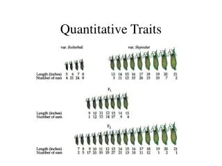
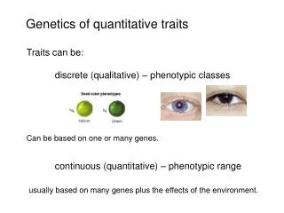
Description All traits fall into a few distinct classes. These classes can be used to predict the genotypes of the individuals. For example, if we cross a tall and short pea plant and look at F2 plants, we know the genotype of short plants, and we can give a generalized genotype for the tall plant phenotype. Furthermore, if we know the genotype we could predict the phenotype of the plant. These type of phenotypes are called discontinuous traits. Other traits do not fall into discrete classes. Rather, when a segregating population is analyzed, a continuous distribution of phenotypes is found. An example, is ear length in corn. Black Mexican Sweet corn has short ears, whereas Tom Thumb popcorn has long ears. When these two inbred lines are crossed, the length of the F1 ears are intermediate to the two parents. Furthermore, when the F1 plants are intermated, the distribution of ear length in the F2 ranges from the short ear Black Mexican Sweet size to the Tom Thumb popcorn size. The distribution resembles the bell-shaped curve for a normal distribution. These are Polygenic Traits:
Description (cont.) Traits that are determined by more than one geneare called continuous traits and cannot be analyzed in the same manner as discontinuous traits. Continuous traits are often measured and given a quantitative value, thus, they are often referred to as quantitative traits. The area of genetics that studies their mode of inheritance is called quantitative genetics.
Description (cont.) • Many important agricultural traits such as: • crop yield, • weight gain in animals, • fat content of meat • are quantitative traits. • Much of the pioneering research into the modes of inheritance of quantitative traits was performed by agricultural geneticists.
Quantitative traits are controlled by multiple genes. Each of thesegenessegregates according to Mendel's laws. Quantitativetraits can also be affected by the environment to varying degrees. e.g. Crop Yield Some Plant Disease Resistances Weight Gain in Animals Fat Content of Meat IQ Learning Ability Blood Pressure
Images of quantitative traits in plants The image demonstrates variation of flower diameter, number of flower parts and the color of the flower Gaillaridiapilchella. Each trait is controlled by a number of genes,thereforeit is a quantitative trait. The photographs demonstratecolorvariability for Indian Paintbrush flower. The parents in the left photo are either yellow or reddish orange. The F2 individuals though show a distribution of colors from yellow to reddish orange. This range of phenotypes is typical of quantitative traits. (This should be compared to flower color of Mendel's peas where the F2 individuals were either purple or white, the two parental phenotypes.)
Genetic and Environmental Effects on Quantitative Traits • If the allelic interactions are known for a particular gene the genotype can be used to predict the phenotype. • With one gene controlling a trait there are three possible genotypes, AA, Aa and aa and depending on the allelic interactions (dominance or incomplete dominance) we can have two or three phenotypes. • As more and more genes control a trait, a greater number of genotypes are possible. The formula that predicts the number of genotypesfrom the number of genes is 3 to the power n. (n is the number of genes.) • The following is the number of genotypes for a selected number (n) of genes which control an arbitrary trait.
Genetic and Environmental Effects on Quantitative Traits The number of genotypes for a selected number (n) of genes which control an arbitrary traitis as follow. # of Genes# of Genotypes 1329 5243 1059,049
Genetic and Environmental Effects on Quantitative Traits (an example) An example with two genes, A and B. When assignedare metric values to each of the alleles. The A allele will give 4 units while the a allele will provide 2 units. At the other locus, the B allele will contribute 2 units while the b allele will provide 1 units. With two genes controlling that trait, nine different genotypes are possible.
Genetic and Environmental Effects on Quantitative Traits (an examplecont.) The genotypes and their associated metric values No. Genotype Ratio in F2 Metric value • AABB 1 12 • AABb2 11 • AAbb1 10 • AaBB2 10 • AaBb4 9 • Aabb2 8 • aaBB1 8 • aaBb2 7 • aabb1 6
The data distribution from table in previous slide. The bell-shaped curve that is indicative of the normal distribution. This has important implications for the manner in which quantitative traits are analyzed.
Genetic and Environmental Effects on Quantitative Traits (an exampleexplanation) The example demonstrates additive gene action. This means that each allele has a specific value that it contributes to the final phenotype. Therefore, each genotypes has a slightly different metric or quantitative value that results in a distribution (or curve) of metric values.
Genetic and Environmental Effects on Quantitative Traits Other genetic interactions such as dominance or epistasis also affect the phenotype. For example, if dominant gene action controls a trait, than the homozygous dominant and heterozygote will have the same phenotypic value. Therefore, the number of phenotypes is less than for additive gene action. Furthermore, the number of phenotypes that result from a specific genotype will be reduced further if epistatic interactions between several loci affects the phenotype.
Genetic and Environmental Effects on Quantitative Traits Additive, dominance, and epistatic effects can all contribute to the phenotype of a quantitative trait, but generally additive interactions are the most important.
Genetic and Environmental Effects on Quantitative Traits All of mentioned factors are genetic in nature, but the environment also affects quantitative traits. The primary affect of the environment is to change the value for a particular genotype. Using our previousexample, the value for the genotype AaBb might vary from 8-10. This variation would be the result of the different environments in which the genotype was grown. The consequence of this environmental effect is that the distribution even more resembles a normal distribution.
Genetic and Environmental Effects on Quantitative Traits To illustrate the effect of environment on the expression of a genotype, the yields of winter wheat at one North Dakota location (Casselton, ND) during the last ten years are presented. Any year for year variation in yield for any one genotype is largely an effect of the environment.
Genetic and Environmental Effects on Quantitative Traits Yield (bushels/acre) Genotype YearRoughriderSewardAgassiz 1986 47.9 55.9 47.5 1987 63.8 72.5 59.5 1988 23.1 25.7 28.4 1989 61.6 66.5 60.5 1990 0.0 0.0 0.0 1991 60.3 71.0 55.4 1992 46.6 49.0 41.5 1993 58.2 62.9 48.8 1994 41.7 53.2 39.8 1995 53.1 65.1 53.5 Note: All plants in 1990 experienced winter kill. (The data from Dr. Jim Anderson, Dept of Plant Sciences, North Dakota State University, Fargo, ND.)
Genetic and Environmental Effects on Quantitative Traits Thus the phenotype is a sum of the environmental and the genetic effects. Stated in a mathematical format: Phenotype = Genetic Factors + Environmental Factors
Genetic and Environmental Effects on Quantitative Traits One of the goals of quantitative genetics is to measure the contribution of genetic and environmental factors on a specific phenotype. However, the field of quantitative genetics also studies other aspects of quantitative traits.
Genetic and Environmental Effects on Quantitative Traits Questions Studied By Quantitative Geneticists: • What is the genetic and environmental contribution to the phenotype? • How many genes influence the trait? • Are the contributions of the genes equal? • How do alleles at different loci interact: additively? epistatically? • How rapid will the trait change under selection?
Statistics of Quantitative Traits Quantitative traits exhibit a continuous distribution of phenotypes, thus, they cannot be analyzed in the same manner as traits controlled by a few genes. Rather, quantitativetraits are described in terms of statistical parameters.
Statistics of Quantitative Traits The two primary statistics used are the mean and the variance.
Statistics of Quantitative Traits An associated statistic that is also relevant is the standard deviation, because it is in the same units as the mean.
Statistics of Quantitative Traits The mean is the average value of the distribution. The graph on the right demonstrates two distributions with the same mean but different variances. Two distribution can have the same mean, but widely different shapes. A wide distribution suggests a large range of values, whereas, a narrow distribution occurs when the range of observed values is small. The variance is a measure of the variability of the distribution.
Statistics of Quantitative Traits A simple way to describe a distribution is in terms of its mean and its standard deviation. The mean ± one standard deviation encompasses ~66% of the distribution. Thus a larger standard deviation suggests that the distribution is wider than one with a smaller standard deviation. Furthermore, ~95% of the distribution is found within ± two standard deviations of the mean and ~99% of the distribution is found within ± three standard deviations. Quantitative genetics of ear length in corn Generation Mean Standard (cm) deviation (cm) Tom Thumb (P1) 16.80 0.816 BMS (P2) 6.63 1.887 F1 12.12 1.519 F2 12.89 2.252
Statistics of Quantitative Traits Several observations can be made from the example. • Even though the mean ear length of the BMS is smaller, the standard deviation is larger. This suggests that it is more variable than the long ear line. • Because the F1 population is derived from two pure lines, it should be entirely homogeneous (all are heterozygotes). Thus all the variance associated with that population is environmental variance. • The mean of a quantitative trait in a F1 population is intermediate to the two parents, and the mean of the F2 is approximately equal to that of the F1. • The F2 population is more variable than the F1. • The extreme values of the distribution should be equivalent to the two parents used in the cross because this small portion of the population will have the same genotypes as the parents. If two genes control the trait 1/16 of the F2 populations will equal either of the two parents. If five genes control the trait then 1/243 of the F2 populations will equal either parent.
Variance Components of a Quantitative Trait The metric value (or phenotypic value) for a specific individual, is the result of genetic factors, environmental factors, and the environmental factors that interact with the genetic factors. The sum of these factors in a population of individuals segregating fora quantitative trait contributes to the variance of that population.
Variance Components of a Quantitative Trait The total variance can be partitioned in the following manner. VP = VG + VE + VGE where, VP= total phenotypic variation of the segregating populationVG= genetic variation that contributes to the total phenotypic variationVE= environmental contribution to the total phenotypic variationVGE= variation associated with the genetic and environmental factor interactions
Variance Components of a Quantitative Trait The genetic variation can be further subdivided into three components. 1. Additive genetic variation. Some alleles may contribute a fixed value to the metric value of quantitative trait. For example, if genes A and B control corn yield (it is actually controlled by many genes), and each allele contributes differently to yield in the following manner:
Variance Components of a Quantitative Trait If genes A and B control corn yield (it is actually controlled by many genes), and each allele contributes differently to yield in the following manner: A = 4 bu/ac a = 2 bu/ac B = 6 bu/ac b = 3 bu/ac
Variance Components of a Quantitative Trait AABB genotype will have a yield of 20 (4+4+6+6) bu/ac The AaBb genotype will yield 15 (4+2+6+3) bu/ac. Genes that act in this manner are additive, and they contribute to the additive genetic variance (VA).
Variance Components of a Quantitative Trait 2. Dominant genetic variance (VD). In addition to genes which have an additive effect on the quantitative trait, other genes may exhibit a dominant gene action which will mask the contribution of the recessive alleles at the locus. If the twosuch genes exhibiting dominance the metric value of the AaBb heterozygote would be 20 bu/ac. This value equals the homozygous dominant genotype in the example where the alleles were acting additively. This source of variability is attributed to the dominance genetic variance (VD).
Variance Components of a Quantitative Trait Interaction genetic variance (VI). This final type of genetic variance is associated with the interactions between genes. The genetic basis of this variance is epistasis, and it is called the interaction genetic variance (VI).
Variance Components of a Quantitative Trait The total genetic variance can be partitioned into the three forms of variance VG = VA + VD + VI The total phenotypic variance can be rewritten as VP = VA + VD + VI + VGE + VGE
Variance Componentsof a Quantitative TraitCONCLUDING By performing specific experiments, quantitative geneticists can estimate the proportion of the total variance that is attributable to the total genetic variance and the environmental genetic variance. If geneticists are trying to improve a specific quantitative trait (such as crop yield or weight gain of an animal), estimates of the proportion of these variances to the total variance provide direction to their research. If a large portion of the variance is genetic, then gains can be made from selecting individuals with the metric value you wish to obtain. On the other hand if the genetic variance is low, which implies that the environmental variance is high, more success would be obtained if the environmental conditions under which the individual will be grown are optimized.
Heritability Broad-sense heritability Itis the ratio of total genetic variance to totalphenotypic variance. H2 = VG/VP Narow-sense heritability Itis the ratio of additive genetic variance to the total phenotypic variance. h2 = VA/VP
Heritability • The heritability estimate is specific to the population and environment which is analyzed. • The estimate is a population, not an individual parameter. • Heritability does not indicate the degree to which a trait is genetic, it measures the proportion of the phenotypic variance that is the result of genetic factors.
Estimating the OffspringPhenotype If the narrow sense heritability of a trait has been determined and several population values is known the phenotypic value for an offspring can be estimated. The following formula can be used for the prediction. To = T + h2(T*-T) Where: To = predicted offspring phenotypeT = population meanh2 = narrow sense heritabilityT* = midparent value [(Tf + Tm)/2]
Estimating the Offspring Phenotype An Example T = 80 seeds/plantTf = 90 seeds/plantTm = 120 seeds/plantT* = (90 +120)/2 = 105h2 = 0.5 Then: To = 80 + 0.5 (105-80)To = 80 + 12.5To = 92.5 seeds/plant
Estimating the Offspring Phenotype The conclusion is not that each plant in the next generation will have 92.5 seeds/plant, but rather that on average the population derived from mating these two parents will have 92.5 seeds/plant. IMPORTANT! The quantitative traits are affected by the environment, and the environment will be responsible for the deviations that one would see from the estimated phenotype.
Predicting Response to Selection Another use of heritability is to determine how a population will respond to selection. Typically parents with the phenotypic value of interest are selected from a base population. These parents are crossed, and a new population is developed.
Predicting Response to Selection The distributions shown on right illustrate this point.
Predicting Response to Selection The selection differential is the difference of the base population mean and the mean of the selected parents. The selection response is how much gain one make when mating the selected parents. IMPORTANT! The narrow sense heritability is a measure of the genetic component that is contributed by the additive genetic variance. The response to selection can thus be derived by multiplying the heritability by the selection differential.
Predicting Response to Selection EXAMPLE The base sunflower population has a mean of 100 days to flowering. Two parents were selected that had a mean of 90 days to flowering. The quantitative trait days to flowering has a heritability of 0.2. What would be the mean of a population derived from crossing these two parents? R = h2SR = 0.2(90 - 100) days to floweringR = -2 days The new population mean would therefore be 98 days to flowering (100 days - 2 days).
http://biolmolgen.slam.katowice.pl/ THANK YOU FOR ATTENTION