Economic Optimization Model
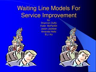
Waiting Line Models For Service Improvement by: Shannon Duffy Katie McPartlin Jason Jacklow Amanda Holtz B.J. Ko. Economic Optimization Model. EOM Which has developed using queuing analysis. EOM. Used at L.L. Bean for telemarketing operations

Economic Optimization Model
E N D
Presentation Transcript
Waiting Line Models For Service Improvementby:Shannon DuffyKatie McPartlinJason JacklowAmanda HoltzB.J. Ko
Economic Optimization Model • EOM • Which has developed using queuing analysis
EOM • Used at L.L. Bean for telemarketing operations • To determine the optimal number of telephone trunks for incoming calls • The number of agents scheduled • The queue capacity • The maximum number of customers who are put on hold to wait for an agent
Queuing models are used • To determine the economic impact of busy signals • Customer waiting time • Lost orders
Decision about waiting lines • Are based on averages for customer arrivals and service times • They are used to computer operation characteristics • Which are average of values for characteristics that describe the performance of a waiting line system
Elements of a waiting line • Basic element is queue • Which is a single waiting line • Which consists of arrivals, servers, and waiting line structure • Single-channel queuing system
The Calling Population • Is the source of the customers to the queuing system, and it can be either infinite or finite • Infinite • Calling population assumes such a large number of potential customers that is always possible for one more customer to arrive to be served • Ex. – grocery store, bank
Finite calling population • Has a specific, countable number of potential customers • Ex. – repair facility in a shop
Arrival Rate • Is the rate at which customers arrive at the service facility during a specified period of time • This rate can be estimated from empirical data derived from studying the system or a similar system, or it can be average of these empirical data
Service times • The time required to serve a customer, is more frequently described by the negative exponential distribution • Service must be expressed as a rate to be compatible with the arrival rate • Customers must be served faster than they arrive or an infinitely large queue will build up
Queue Discipline and Length • Queue discipline is the order in which waiting customers are served • Most common type is first come, first served
Infinite Queue • Can be of any size with no upper limit and is the most common queue structure • Ex. Movie theater line
Finite Queue • Is limited to size • Ex. Driveway at bank
Basic Waiting Line Structures • There are four basic structures according to the nature of the service facilities • Single-channel, single-phase • Single-channel, multiple-phase • Multiple-channel, single-phase • Multiple-channel, multiple-phase
Channels and Phases • Channel • Is the number of parallel servers for servicing arriving customers • Phases • Denotes the number of sequential servers each customer must go through to complete service
Poisson Distribution • The Poisson Distribution is a discrete distribution which takes on the values X=0,1,2,3… • It is often used as a model for the number of events (such as the number of telephone calls at a business or the number of accidents at an intersection) in a specific time period.
Single-Channel, Single-Phase Models • Most basic of the waiting line structures • Frequently used variation • Poisson arrival rate, exponential service times • Poisson arrival rate, general distribution of service times • Poisson arrival rate, constant service items • Poisson arrival rate, exponential service times with a finite queue and a finite calling population
Basic Single-Server Model • Assume the following • Poisson arrival rate • Exponential service times • First-come, first-served queue discipline • Infinite queue length • Infinite calling population
Constant Service times • The single-server model with Poisson arrivals and constant service times is a queuing variation that is of particular interest in operations management, since the most frequent occurrence of constant service times is with automated equipment and machinery. • This model has direct applications for many manufacturing operations
Finite Queue Length • Since some waiting lines systems the length of the queue may be limited by the physical area in which the queue forms; • Space may permit only a limited number of customers to enter the queue • Variation of the single-phase, single-channel queuing model
Finite Calling Populations • The population of customers from which arrivals originate is limited, such as the number of police cars at a station to answer calls
Multi-Server Models • Two or more independent servers in parallel serve a single waiting line • The number of servers must be able to serve customers faster than they arrive
Definition of Variables • Pn = Probability of n Units in System • = Mean Number of Arrivals per Time Period • = Mean Number of People or Items Served per Time Period • Ls = Average Number of Units in the System • Ws = Average Time a Unit Spends in the System (Wait Time + Service Time)
Definition of VariablesContinued • Lq = Average Number of Units in the Waiting Line • Wq = Average Time a Unit Spends Waiting in the Line • = Utilization Factor for the System (Percent of Time the Servers are Busy) • P0 = Probability of 0 Units in the System
Single Channel, Single Phase • Ls = /( • Ws = 1/( • Lq = • Wq = • • P0 = • Pn =n • In all Cases,
Single Channel, Single Phase Example • For cars arriving/hour • cars serviced/hour • Ls = /(= 2/(3-2) = 2 cars in System • Ws = 1/(= 1/(3-2) = 1 hour average time spent in system • Lq == 22/3(3-2) = 1.33 cars waiting
Single Channel, Single Phase Example Cont. • Wq = = 2/(3(3-2)) = 2/3 hour or 40 minute average time waiting • = 2/3 = 66.7% Utilization of Mechanic • P0 = = 1-(2/3) = 1/3 = 0.33 probability there are no cars in system = 0.33 • P1 =1 = (2/3)12/3)) = 1/9 probability there is 1 car in system = 0.11
The End Any Questions?

