Image Processing
Image Processing. Chapter 14. Landsat 7 image of the retreating Malaspina Glacier, Alaska. Image Basics. Earth science is a very visual discipline Graphs Maps Field Photos Satellite images Because of this, all Earth scientists should have: Basic knowledge about graphics file types
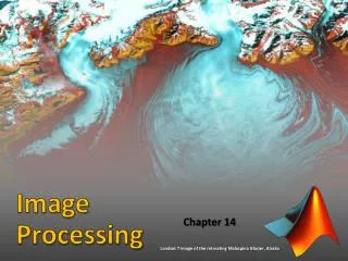

Image Processing
E N D
Presentation Transcript
Image Processing Chapter 14 Landsat 7 image of the retreating Malaspina Glacier, Alaska
Image Basics • Earth science is a very visual discipline • Graphs • Maps • Field Photos • Satellite images • Because of this, all Earth scientists should have: • Basic knowledge about graphics file types • Pros/cons of different graphics file types Landsat image of Death Valley, CA Cathodoluminescence image of granite Sediment Core Siccar Point: The first recognized angular unconformity by James Hutton Image: Chris Rowan @ Highly Allochthonous Blog Photomicrograph of peridotite (mantle rock) NED Dataset
Image File Types: Raster vs Vector Raster Image • Made of pixels • When you scale it, quality changes (finite # pixels) • Common formats: jpg, png, gif, tif, bmp Vector Image • Made of vector objects (not pixel-based) • Can scale to any size • Common Formats: ai, eps, ps, svg, wmf, pdf Many Formats Can Contain Both Vector and Raster Images • For example, ai, pdf, eps, ps, wmf • How can you tell? Zoom in on the image • Which is better? • Depends on use • For graphs/plots: typically vector (unless data set is HUGE) • For photos: raster
Zoomed In… • Raster images are made of square pixels • Each pixel has a single and constant color
Image Processing in MATLAB • MATLAB provides functions that read raster images • Each pixel’s value (color) is stored as a number in matrix • MATLAB also has an image processing toolbox with TONS of image processing options. • In this class, we will only use the image functions that are part of the standard MATLAB libraries • imread, image, imagesc, colormap, Landsat false-color image examples… Yukon River delta, Alaska Mississippi River meanders & oxbows near Memphis, TN Novarupta Volcano, Aleutian Islands, Alaska Purples/Reds: Volcanic ash from 1912 Eruption Blues: Snow/Ice
Color Models • Before we start processing images, we need to talk about how computers represent colors as numbers • Three common color models • RGB: An additive model • works like light • CMYK: A subtractive model • works like ink • HSV: A cone-shaped model • useful for shading colors
The RGB Color Model • For variables of class uint8 (and 8-bit images) • 0-255 are the possible integer values (same for the uint8 class!) • 0 is minimum for any RGB color • 255 is max for any RGB color • To define any color, you must specify the Red (R), Green (G), and Blue (B)values • Wait, color can be a vector! • Grayscale images only need one value (0=black, 255=white) [ 0 0 0 ] [ 255 255 255 ] [ 75 75 75 ] [ 200 200 200] [ 255 0 0] [ 100 0 0] [ 0 255 0] Total number of different colors: 2563 = 16,777,216 [ 0 100 0 ] [ 0 0 255 ] [ 0 0 100 ] [ 255 255 0] [ 0 255 255] [ 255 0 255] [ 237 125 49]
Colormaps in MATLAB • Just to annoy us, MATLAB requires colormap RGB values to be values between 0 and 1 for variables of class double • 0 is minimum for any RGB color • 1 is max for any RGB color • To define any color, you must specify the Red (R), Green (G), and Blue (B)values • To convert from the 0-255 system, just divide by 255! Or cast as uint8 • Grayscale images really only need one value (0=black, 1=white) [ 0 0 0 ] [ 1 1 1 ] [ 0.29 0.29 0.29 ] [ 0.78 0.78 0.78] [ 1 0 0] [ 0.39 0 0] [ 0 1 0] [ 0 0.39 0 ] [ 0 0 1 ] [ 0 0 0.39 ] [ 1 1 0] [ 0 1 1] [ 1 0 1] [ 0.93 0.49 0.19]
MATLAB & Images MATLAB can represent color in images in two basic ways • True Color or RGB • The three color components are stored in a m x n x 3 matrix. I.e. a 3D matrix. (:, :, 1) R-values; (:, :, 2) G-values; (:, :, 3) B-values • Indexed to a Colormap • Colors are stored as a single integer value that corresponds to a row in a colormap matrix. • Colormap stores the RGB values 4 Pixel Image Colormap Matrix Image Matrix
Images Represented as Colormaps • ‘image’ plots a matrix as an image • Don’t forget to specify the colormap • If not, you get the default 64 color ‘jet’ colormap
Built-In Colormaps • MATLAB provides several built-in colormaps • The command colormap is rather useful • It can set the current colormap • Can be a built-in map or a custom n x 3 matrix • Built-in colormaps can be easily scaled • E.g. “jet(256)” returns a 256 x 3 matrix that follows the color scheme of the built-in “jet” colormap.
True Color Images If ‘image’ is passed a 3D matrix • It is assumed to be a true color image • 1st level R-values • 2nd level G-values • 3rd level B-values If ‘image’ is passed a 2D matrix • It is assumed to be an colormap indexed image
Exceed Max/Min Indexed Color? • If you exceed the color map values, you get either the min or max color
Why have both Types of Images? Why does MATLAB offer two ways to store image colors? • Flexibility. It is always good to give users options • Grayscale vs Color Images • These images are typically read in MATLAB in different ways • Grayscale: Indexed Color • Color image: True Color or RGB image
Reading in Grayscale Images • ‘imread’ can read in most standard grayscale raster image types • .jpg .gif .png, etc… • Stores image as a rectangular matrix • Each entry represents one pixel’s grayscale value • 0-255 (black to white) • Let’s read this image into MATLAB • The image is 814 x 531 pixels • Matrix will be 531 x 814 • Try to automate detection of the dendrites Cropped grayscale image of dendrites Increased contrast (using Photoshop)
Reading in Grayscale Images • If ‘image’ is given a 2D matrix, it assumes the image is indexed color
Reading in Grayscale Images How could I figure out the % dendrites?
Reading in True Color / RGB Images Landsat image of Yukon River delta • ‘imread’ can read in most standard RGB raster image types • .jpg .gif .png, etc… • Stores image as a 3D matrix • Each entry represents one pixel’s R, G, or B value • 0-255 (min/max) • 1st z-slice = Red values • 2nd z-slice = Green values • 3rd z-slice = Blue values • Let’s read this image into MATLAB • The image is 1000 x 1001 pixels • Matrix will be 1001 x 1000 x 3 • Try to automate detection of the water Google Earth Image (aerial photo)
Reading in True Color / RGB Images • Are all of the selected pixels actually blue? (No) • How could I improve water detection? • How could I calculate water surface area?
Final Thoughts… • Images are everywhere in Earth sciences • Images are actually matrices of numbers • MATLAB can be used to automate detection of features in images. • Can replace point counting • Saves time!